Rifampicin (Gafar 2026)
Source:vignettes/articles/Gafar_2026_rifampicin.Rmd
Gafar_2026_rifampicin.RmdModel and source
mod <- rxode2::rxode(readModelDb("Gafar_2026_rifampicin"))
#> ℹ parameter labels from comments will be replaced by 'label()'
#> Warning: some etas defaulted to non-mu referenced, possible parsing error: etaiov_fdepot_1, etaiov_fdepot_2, etaiov_ka_1, etaiov_ka_2, etaiov_mtt_1, etaiov_mtt_2
#> as a work-around try putting the mu-referenced expression on a simple line- Citation: Gafar F., Svensson E. M., Yunivita V., Fregonese F., Fisher D., Fox G. J., Nguyen T. A., Nguyen B. H., Johnston J., Long R., Valiquette C., Aarnoutse R. E., Ruslami R., Menzies D. (2026). Population Pharmacokinetic Modeling of Standard- and High-Dose Rifampicin for Tuberculosis Preventive Therapy in the 2R2 Randomized Controlled Trial. The Journal of Infectious Diseases 233(4):e999-e1010. doi:10.1093/infdis/jiag052. Parameter estimates from Table 2; model equations from the Figure 1 caption and from the NONMEM control stream reproduced verbatim in Supplementary Appendix 1. The saturable-hepatic-extraction structure was adapted from Chirehwa et al. (2016) Antimicrob Agents Chemother 60(1):487-494 doi:10.1128/AAC.01830-15, with autoinduction omitted because sampling was performed only once at week 4. Fat-free mass follows Janmahasatian et al. (2005) Clin Pharmacokinet 44(10):1051-1065 doi:10.2165/00003088-200544100-00004.
- Article: J Infect Dis 2026;233(4):e999-e1010
- Supplement:
jiag052_supplementary_data.pdf(Tables S1-S7, Figures S1-S2 and Appendix 1, the complete NONMEM control stream of the final model), published with the open-access article (PMC13127750).
Rifampicin is cleared almost entirely by the liver, and at the doses
used for tuberculosis preventive therapy that clearance saturates. Gafar
2026 therefore does not fit an apparent CL/F; it fits a
well-stirred liver sitting between the gut and the
systemic circulation:
The absorbed dose is delivered into the liver, so
first-pass extraction is structural rather than a fitted F
term, and the drug recirculates from the central compartment back to the
liver with hepatic blood flow. As the dose goes up,
rises,
falls,
falls, and both the systemic clearance
and the first-pass loss
shrink at the same time. That double effect is what produces the
greater-than-proportional exposure the paper reports: the median
AUC0-24 is 2.5-fold higher at 20 mg/kg and 4-fold higher at
30 mg/kg than at 10 mg/kg.
Absorption is a Savic analytical transit chain (NN = 17.9, MTT = 0.768 h) feeding a first-order absorption compartment.
Population
The model was built on 1041 rifampicin concentrations from 440 adolescents and adults with tuberculosis infection enrolled in the 2R2 phase 2b randomized trial (NCT03988933) at seven sites in Canada, Indonesia and Vietnam. Median age was 40 years (IQR 26-50; 7.3% were adolescents aged 10-17 years), median body weight 60.0 kg (IQR 51.0-71.0), median fat-free mass 41 kg (IQR 35.3-49.2) and 57.9% were female (source Table 1). Most participants were Indonesian (265, 60.2%), with 87 (19.8%) Canadian and 88 (20.0%) Vietnamese.
Unlike almost every other published rifampicin population PK model, this cohort is generally healthy - these are people with latent tuberculosis infection, not tuberculosis disease. The paper’s Table S6 shows the consequence: at every dose level the 2R2 exposures run 1.1- to 3.6-fold above the values reported in tuberculosis-disease cohorts.
Participants were randomized to 10 mg/kg/day for 120 days (4R10) or to 20 or 30 mg/kg/day for 60 days (2R20, 2R30), dispensed by the prespecified weight bands of Table S3. Because the highest band was open-ended (>55 kg), heavier participants received lower-than-intended mg/kg doses, so the popPK treatment arms were redefined by the actual dose received: 5.1-15.0 mg/kg (n = 191), 15.1-25.0 mg/kg (n = 159) and 25.1-35.0 mg/kg (n = 90). Sampling was performed at approximately 4 weeks of treatment (median 30 days), assumed to be steady state and past the completion of rifampicin autoinduction - which is why the autoinduction component of the reference model was dropped.
The same information is available programmatically via
readModelDb("Gafar_2026_rifampicin")()$population.
Source trace
Every ini() value carries an in-file comment pointing at
its origin. Because the complete NONMEM control stream is published as
Supplementary Appendix 1, each value can be traced twice: to the printed
Table 2 row and to the $THETA / $OMEGA entry
it came from. The two agree everywhere except the two residual-error
rows (see Assumptions and deviations).
| Equation / parameter | Value | Source location |
|---|---|---|
lclint_max |
46.7 L/h | Table 2 “Intrinsic clearance, CL int,max”;
$THETA (0, 46.7) ;[CL]
|
lvc |
22.8 L | Table 2 “Volume of distribution, V”;
$THETA (0, 22.8) ;[V]
|
lka |
4.38 /h | Table 2 “Absorption rate constant, Ka” (4.4);
$THETA (0, 4.38) ;[KA]
|
lmtt |
0.768 h | Table 2 “Mean transit time, MTT” (0.8);
$THETA (0, 0.768) ;[MTT]
|
lnn |
17.9 | Table 2 “Number of transit compartments, NN”;
$THETA (0, 17.9) ;[NN]
|
lfdepot |
1 fixed | Table 2 “Prehepatic bioavailability, F: 1 fixed”;
$THETA (1) FIX ;[BIO]
|
lkm |
4.16 (log scale) | Table 2 “Michaelis-Menten constant, Km = 64.1 mg/L” with footnote d
“Km was log-transformed during estimation”;
$THETA (0, 4.16) ;[LOGKM], exp(4.16) = 64.07 |
lqh |
90 L/h fixed | Table 2 “Hepatic blood flow, QH: 90 fixed”;
$THETA (90) FIX ;[QH]
|
lvh |
1 L fixed | Table 2 “Volume of distribution of the hepatic compartment, VH: 1
fixed”; $THETA (1) FIX ;[VH]
|
fub |
0.2 fixed | Table 2 “Unbound fraction of rifampicin, fu: 0.2 fixed”;
$THETA (0.2) FIX ;[FU]
|
e_ffm_clint_max, e_ffm_qh
|
0.75 fixed | Methods “Covariate Model”: “power exponents fixed at 0.75 for
clearance”; $PK ALLMCL = (FFM/41)**0.75,
QH = THETA(7)*(FFM/56)**0.75
|
e_ffm_vc, e_ffm_vh
|
1 fixed | Methods “Covariate Model”: “and 1 for volume parameters”;
$PK ALLMV = (FFM/41)**1,
VH = THETA(9)*(FFM/56)
|
e_region_canada_fdepot |
0.782 | Table 2 “Formulation used in Canada versus Indonesia: -21.8%”;
$THETA (0, 0.782) ;[BIOFRM1]
|
e_region_vietnam_fdepot |
0.877 | Table 2 “Formulation used in Vietnam versus Indonesia: -12.3%”;
$THETA (0, 0.877) ;[BIOFRM2]
|
etalclint_max |
var 0.0137 | Table 2 “BSV in CL 11.7 CV%”;
$OMEGA 0.0137 ;[IIV in CL]
|
etalvc |
var 0.0221 | Table 2 “BSV in V 14.9 CV%”;
$OMEGA 0.0221 ;[IIV in V]
|
etalkm |
var 0.0213 | Table 2 “BSV in Km 14.7 CV%”;
$OMEGA 0.0213 ;[IIV in LOGKM]
|
etaiov_fdepot_1/2 |
var 0.0421 | Table 2 “BOV in F 20.7 CV%”; $OMEGA BLOCK(1) 0.0421 +
SAME
|
etaiov_ka_1/2 |
var 1.18 | Table 2 “BOV in Ka 150.1 CV%”; $OMEGA BLOCK(1) 1.18 +
SAME
|
etaiov_mtt_1/2 |
var 0.176 | Table 2 “BOV in MTT 43.9 CV%”; $OMEGA BLOCK(1) 0.176 +
SAME
|
propSdSparse |
0.116 |
$THETA (0, 0.116) ;[PROP-ITS0]; Table 2 prints 35.1
(see erratum below) |
propSdIntensive |
0.187 |
$THETA (0, 0.187) ;[PROP-ITS1]; Table 2 prints 45.3
(see erratum below) |
addSd |
0.025 mg/L fixed | Table 2 “Additive, mg/L: 0.025 fixed” with footnote e;
$ERROR ADD = LLOQ/5 + THETA(15) with LLOQ 0.125 and
$THETA (0) FIX
|
d/dt(depot), d/dt(liver),
d/dt(central)
|
n/a | Figure 1 caption (equations for CLH, EH, CLint, ktr) and
$DES DADT(1)-DADT(3) of Appendix 1 |
transit(nn, mtt, fdepot) |
n/a |
$PK PIZZA = LOG(BIO*PD*KTR+0.00001)-GAMLN(NN+1) with
$DES TRANSIT = EXP(PIZZA+NN*LOG(KTT)-KTT),
KTR = (NN+1)/MTT (Figure 1 caption) |
| FFM (Janmahasatian) | n/a | Table 1 footnote a / Table S4 footnote a |
Structural identities
These checks compare the solved model against closed forms derived from the same drawn parameters, so the only error is numerical and the tolerances are tight.
tv <- rxode2::zeroRe(mod)
#> Warning: some etas defaulted to non-mu referenced, possible parsing error: etaiov_fdepot_1, etaiov_fdepot_2, etaiov_ka_1, etaiov_ka_2, etaiov_mtt_1, etaiov_mtt_2
#> as a work-around try putting the mu-referenced expression on a simple line

# `ndose` daily doses, observing over the last dosing interval.
solve_one <- function(dose, FFM, ca = 0, vn = 0, grid = seq(0, 24, by = 0.01),
                      ndose = 7L) {
  start <- 24 * (ndose - 1L)
  d <- data.frame(
    id = 1L, time = c(0, start + grid), evid = c(1L, rep(0L, length(grid))),
    amt = c(dose, rep(NA_real_, length(grid))),
    cmt = c("depot", rep("central", length(grid))),
    ii = c(24, rep(0, length(grid))),
    addl = c(ndose - 1L, rep(0L, length(grid)))
  )
  d$FFM <- FFM
  d$REGION_CANADA <- ca
  d$REGION_VIETNAM <- vn
  d$OCC <- 1
  d$SAMPLE_INTENSIVE <- 0
  # method = "lsoda": rxode2's default liblsoda returns "could not solve the
  # system" on the dense (<= 0.005 h) observation grids used below, while
  # lsoda and dop853 both solve them and agree to every printed digit. The
  # grid has to be dense here because the transit chain produces a feature
  # about 0.17 h wide and these checks are integrated by trapezoid.
  s <- rxode2::rxSolve(tv, d, returnType = "data.frame", method = "lsoda")
  s <- s[!is.na(s$Cc) & s$time >= start, ]
  s$tad <- s$time - start
  s
}

trapz <- function(x, y) sum(diff(x) * (utils::head(y, -1) + utils::tail(y, -1)) / 2)

## (1) Steady-state hepatic mass balance. Over one dosing interval at steady
##     state the amount eliminated by the liver, integral(k20 * A_liver) dt,
##     must equal the amount that entered, fdepot * dose.
mb <- solve_one(dose = 600, FFM = 41)
#> ℹ omega/sigma items treated as zero: 'etalclint_max', 'etalvc', 'etalkm', 'etaiov_fdepot_1', 'etaiov_fdepot_2', 'etaiov_ka_1', 'etaiov_ka_2', 'etaiov_mtt_1', 'etaiov_mtt_2'
eliminated <- trapz(mb$tad, mb$k20 * mb$liver)
mass_balance_err <- abs(eliminated - 600) / 600

## (2) Linear-limit closed form. At a dose small enough that C_H << Km the
##     intrinsic clearance is CLint,max, so the systemic clearance is Q_H E_H0
##     and the oral availability is (1 - E_H0):
##        AUC = dose * (1 - E_H0) / (Q_H * E_H0)
lin <- solve_one(dose = 1, FFM = 41, grid = seq(0, 24, by = 0.002))
#> ℹ omega/sigma items treated as zero: 'etalclint_max', 'etalvc', 'etalkm', 'etaiov_fdepot_1', 'etaiov_fdepot_2', 'etaiov_ka_1', 'etaiov_ka_2', 'etaiov_mtt_1', 'etaiov_mtt_2'
qh0  <- 90 * (41 / 56)^0.75
eh0  <- (46.7 * 0.2) / (46.7 * 0.2 + qh0)
auc_closed <- 1 * (1 - eh0) / (qh0 * eh0)
auc_solved <- trapz(lin$tad, lin$Cc)
linear_err <- abs(auc_solved - auc_closed) / auc_closed

## (3) Saturation direction: exposure must rise faster than proportionally.
d10 <- solve_one(600, 41)
#> ℹ omega/sigma items treated as zero: 'etalclint_max', 'etalvc', 'etalkm', 'etaiov_fdepot_1', 'etaiov_fdepot_2', 'etaiov_ka_1', 'etaiov_ka_2', 'etaiov_mtt_1', 'etaiov_mtt_2'
d20 <- solve_one(1200, 41)
#> ℹ omega/sigma items treated as zero: 'etalclint_max', 'etalvc', 'etalkm', 'etaiov_fdepot_1', 'etaiov_fdepot_2', 'etaiov_ka_1', 'etaiov_ka_2', 'etaiov_mtt_1', 'etaiov_mtt_2'
d30 <- solve_one(1800, 41)
#> ℹ omega/sigma items treated as zero: 'etalclint_max', 'etalvc', 'etalkm', 'etaiov_fdepot_1', 'etaiov_fdepot_2', 'etaiov_ka_1', 'etaiov_ka_2', 'etaiov_mtt_1', 'etaiov_mtt_2'
auc <- vapply(list(d10, d20, d30), function(s) trapz(s$tad, s$Cc), numeric(1))

## (4) Accumulation. The terminal half-life is about 1.9 h against a 24 h
##     dosing interval, so the seventh dose should look like the first. This
##     is what licenses simulating the cohort below over a single dosing
##     interval instead of integrating seven days per subject.
first_dose <- vapply(c(600, 1200, 1800), function(dz) {
  s <- solve_one(dz, 41, ndose = 1L)
  trapz(s$tad, s$Cc)
}, numeric(1))
#> ℹ omega/sigma items treated as zero: 'etalclint_max', 'etalvc', 'etalkm', 'etaiov_fdepot_1', 'etaiov_fdepot_2', 'etaiov_ka_1', 'etaiov_ka_2', 'etaiov_mtt_1', 'etaiov_mtt_2'
#> ℹ omega/sigma items treated as zero: 'etalclint_max', 'etalvc', 'etalkm', 'etaiov_fdepot_1', 'etaiov_fdepot_2', 'etaiov_ka_1', 'etaiov_ka_2', 'etaiov_mtt_1', 'etaiov_mtt_2'
#> ℹ omega/sigma items treated as zero: 'etalclint_max', 'etalvc', 'etalkm', 'etaiov_fdepot_1', 'etaiov_fdepot_2', 'etaiov_ka_1', 'etaiov_ka_2', 'etaiov_mtt_1', 'etaiov_mtt_2'
accum <- abs(auc - first_dose) / auc

tibble::tibble(
  Check = c("Hepatic mass balance (relative error)",
            "Linear-limit closed-form AUC (relative error)",
            "AUC ratio 1200/600 mg (proportional would be 2)",
            "AUC ratio 1800/600 mg (proportional would be 3)",
            "Accumulation, dose 7 vs dose 1 AUC (largest relative difference)"),
  Value = c(signif(mass_balance_err, 3), signif(linear_err, 3),
            round(auc[2] / auc[1], 3), round(auc[3] / auc[1], 3),
            signif(max(accum), 3))
) |>
knitr::kable(caption = "Structural identity checks on the solved model.")| Check | Value |
|---|---|
| Hepatic mass balance (relative error) | 0.0000003 |
| Linear-limit closed-form AUC (relative error) | 0.0003220 |
| AUC ratio 1200/600 mg (proportional would be 2) | 2.3260000 |
| AUC ratio 1800/600 mg (proportional would be 3) | 3.9800000 |
| Accumulation, dose 7 vs dose 1 AUC (largest relative difference) | 0.0010200 |
stopifnot(
  # Deterministic: identical parameters on both sides, so this is pure
  # trapezoidal error and a tight bound is correct.
  mass_balance_err < 1e-3,
  linear_err < 5e-3,
  # Saturable hepatic extraction must produce more-than-proportional exposure.
  auc[2] / auc[1] > 2,
  auc[3] / auc[1] > 3,
  # A single dosing interval is within 0.5% of steady state.
  max(accum) < 5e-3
)
The extraction ratio is the mechanism, so it is worth seeing directly: at the median fat-free mass of 41 kg, falls from 0.116 at vanishing concentration to markedly less than that across a 30 mg/kg peak.
ch <- seq(0, 400, length.out = 400)
eh_curve <- tibble::tibble(
  c_liver = ch,
  eh = ((46.7 * exp(4.16) / (ch + exp(4.16))) * 0.2) /
    ((46.7 * exp(4.16) / (ch + exp(4.16))) * 0.2 + qh0)
)
peaks <- vapply(list(d10, d20, d30), function(s) max(s$liver / (41 / 56)), numeric(1))
ggplot(eh_curve, aes(c_liver, eh)) +
  geom_line(linewidth = 0.8) +
  geom_vline(xintercept = peaks, linetype = "dashed", colour = "grey40") +
  labs(x = "Liver concentration (mg/L)", y = expression(E[H])) +
  theme_bw()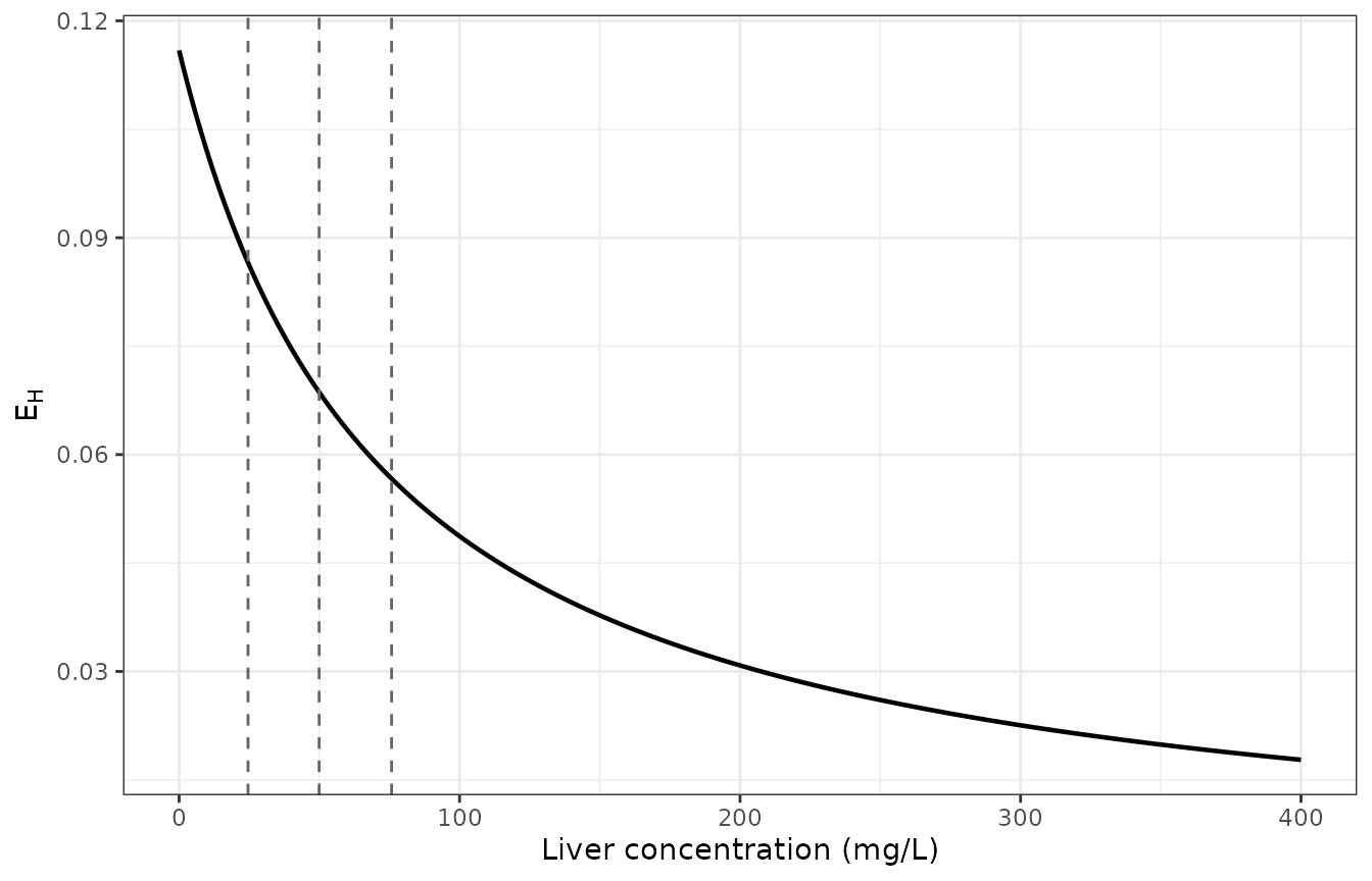
Hepatic extraction ratio as a function of liver concentration at FFM = 41 kg. The dashed lines mark the peak liver concentrations reached at 600, 1200 and 1800 mg.
Virtual cohort
The original data are not publicly available. The cohort below reproduces the 2R2 design: three countries, three randomized arms, weight-band dosing from Table S3, and per-country body-weight distributions from Table S7. Fat-free mass is derived with the Janmahasatian formula exactly as the source paper does.
One step matters more than it looks. The published analysis re-labelled every participant by the dose they actually received (5.1-15.0, 15.1-25.0 and 25.1-35.0 mg/kg), because the top weight band was open-ended, so a heavy participant randomized to 30 mg/kg could receive well under 25 mg/kg. The cohort below applies the same rule to the drawn weights. Skipping it leaves each simulated arm contaminated with subjects the paper would have moved elsewhere, which biases the low arms up and the high arms down by roughly 15%. It also reproduces, from the design alone, the paper’s most awkward result: so few Canadian participants actually reached 30 mg/kg that Table 3 reports that cell as a two-subject range.
set.seed(20260901)
rxode2::rxSetSeed(20260901)  # common random numbers for the eta draws

N_PER_GROUP <- 30L  # 30 per country x randomized arm, well under the 200/arm cap

# Log-normal parameters from a median and an interquartile range.
lnorm_from_iqr <- function(med, q1, q3) {
  c(meanlog = log(med), sdlog = (log(q3) - log(q1)) / (2 * stats::qnorm(0.75)))
}

# Table S7: per-country body weight median (IQR).
wt_par <- list(
  Canada    = lnorm_from_iqr(73.8, 64.0, 85.4),
  Indonesia = lnorm_from_iqr(58.1, 50.0, 69.5),
  Vietnam   = lnorm_from_iqr(57.0, 51.0, 63.0)
)
# Table 1: cohort body mass index median 24.1 (IQR 20.7-27.8).
bmi_par <- lnorm_from_iqr(24.1, 20.7, 27.8)

# Table S3 weight-band daily dose (mg) by arm.
band_dose <- function(wt, arm) {
  band <- ifelse(wt <= 35, 1L, ifelse(wt <= 55, 2L, 3L))
  doses <- matrix(c(300, 450, 600, 600, 900, 1200, 900, 1350, 1800),
                  nrow = 3, dimnames = list(NULL, c("10", "20", "30")))
  doses[cbind(band, match(as.character(arm), colnames(doses)))]
}

janmahasatian <- function(wt, bmi, sexf) {
  ifelse(sexf == 1,
         9270 * wt / (8780 + 244 * bmi),
         9270 * wt / (6680 + 216 * bmi))
}

cohort <- tidyr::expand_grid(
  country = c("Canada", "Indonesia", "Vietnam"),
  target = c(10L, 20L, 30L),
  k = seq_len(N_PER_GROUP)
) |>
  dplyr::mutate(
    id = dplyr::row_number(),
    WT = stats::rlnorm(dplyr::n(),
                       vapply(country, function(x) wt_par[[x]][["meanlog"]], numeric(1)),
                       vapply(country, function(x) wt_par[[x]][["sdlog"]], numeric(1))),
    BMI = stats::rlnorm(dplyr::n(), bmi_par[["meanlog"]], bmi_par[["sdlog"]]),
    SEXF = stats::rbinom(dplyr::n(), 1L, 0.579),
    FFM = janmahasatian(WT, BMI, SEXF),
    REGION_CANADA = as.integer(country == "Canada"),
    REGION_VIETNAM = as.integer(country == "Vietnam"),
    OCC = 1,
    SAMPLE_INTENSIVE = 0,
    dose = band_dose(WT, target),
    mgkg = dose / WT,
    # The source paper's re-classification by actual mg/kg dose received
    # (Results "Participants and Pharmacokinetic Data").
    arm = dplyr::case_when(
      mgkg > 5.1 & mgkg <= 15 ~ 10L,
      mgkg > 15  & mgkg <= 25 ~ 20L,
      mgkg > 25  & mgkg <= 35 ~ 30L,
      TRUE ~ NA_integer_
    )
  ) |>
  dplyr::filter(!is.na(arm)) |>
  dplyr::mutate(grp = paste0(country, " ", arm, " mg/kg")) |>
  dplyr::select(-k)

cohort |>
  dplyr::count(country, arm) |>
  tidyr::pivot_wider(names_from = arm, values_from = n,
                     names_prefix = "n at ", values_fill = 0L) |>
  dplyr::rename(Country = country) |>
  knitr::kable(
    caption = paste(
      "Simulated cohort size by country and actual-dose arm after the source",
      "paper's re-classification. Compare the shape with source Table 1:",
      "Canada contributed 48 / 37 / 2 participants at 10 / 20 / 30 mg/kg."
    )
)| Country | n at 10 | n at 20 | n at 30 |
|---|---|---|---|
| Canada | 43 | 29 | 17 |
| Indonesia | 31 | 34 | 24 |
| Vietnam | 31 | 30 | 29 |
cohort |>
  dplyr::group_by(country) |>
  dplyr::summarise(
    n = dplyr::n(),
    `Body weight (kg)` = sprintf("%.1f (%.1f-%.1f)", stats::median(WT),
                                 stats::quantile(WT, .25), stats::quantile(WT, .75)),
    `Fat-free mass (kg)` = sprintf("%.1f (%.1f-%.1f)", stats::median(FFM),
                                   stats::quantile(FFM, .25), stats::quantile(FFM, .75)),
    `Actual dose (mg/kg)` = sprintf("%.1f (%.1f-%.1f)", stats::median(mgkg),
                                    stats::quantile(mgkg, .25), stats::quantile(mgkg, .75)),
    .groups = "drop"
  ) |>
  dplyr::rename(Country = country, N = n) |>
  knitr::kable(
    caption = paste(
      "Simulated cohort, median (IQR), against the source Table S7 medians:",
      "body weight 73.8 / 58.1 / 57.0 kg and fat-free mass 51.3 / 40.1 / 38.0 kg",
      "for Canada / Indonesia / Vietnam."
    )
)| Country | N | Body weight (kg) | Fat-free mass (kg) | Actual dose (mg/kg) |
|---|---|---|---|---|
| Canada | 89 | 74.9 (64.9-83.7) | 52.3 (45.3-59.4) | 15.6 (9.1-22.4) |
| Indonesia | 89 | 58.3 (48.3-66.9) | 39.5 (32.4-45.0) | 18.3 (10.0-25.5) |
| Vietnam | 90 | 56.9 (52.5-63.8) | 39.9 (35.1-45.1) | 18.6 (10.3-26.8) |
# One common observation grid for every subject: rxSolve cost grows
# superlinearly in the number of pooled subjects, and worse again when they
# carry different time grids. The grid is dense over the absorption window
# because the transit chain produces a feature about 0.17 h wide, and coarse
# after 8 h where the profile is a slow log-linear decline.
grid <- c(seq(0, 4, by = 0.025), seq(4.1, 8, by = 0.1), seq(8.5, 24, by = 0.5))

# A single dosing interval, licensed by identity check (4) above: with a ~1.9 h
# terminal half-life against 24 h dosing, dose 7 and dose 1 differ by ~0.1%.
doses <- cohort |>
  dplyr::transmute(id, time = 0, evid = 1L, amt = dose, cmt = "depot")
obs <- tidyr::expand_grid(id = cohort$id, time = grid) |>
  dplyr::mutate(evid = 0L, amt = NA_real_, cmt = "central")

events <- dplyr::bind_rows(doses, obs) |>
  dplyr::left_join(
    dplyr::select(cohort, id, FFM, REGION_CANADA, REGION_VIETNAM, OCC,
                  SAMPLE_INTENSIVE, grp, country, arm),
    by = "id"
  ) |>
  dplyr::arrange(id, time, dplyr::desc(evid)) |>
  as.data.frame()

sim <- rxode2::rxSolve(mod, events, keep = c("grp", "country", "arm"),
                       returnType = "data.frame") |>
  dplyr::filter(!is.na(Cc)) |>
  # During the absorption lag the true concentration is around 1e-70, and the
  # solver returns round-off of either sign there (values down to -7e-11 were
  # seen). PKNCA's linear-up/log-down trapezoid takes the log of a declining
  # segment, so a single negative round-off turns that subject's AUC into NaN
  # -- silently, and it hit 109 of 268 subjects before this clamp. A negative
  # concentration is numerical noise, not a prediction; clamp it at zero.
  dplyr::mutate(Cc = pmax(Cc, 0), tad = time)
Replicating Figure 2: steady-state concentration-time profiles by dose
Figure 2 of the source is a visual predictive check of observed steady-state concentrations stratified by actual mg/kg dose. Without the observed data the comparison is to the shape and level of the simulated percentiles.
sim |>
  dplyr::group_by(arm, tad) |>
  dplyr::summarise(
    med = stats::median(Cc),
    lo = stats::quantile(Cc, 0.05),
    hi = stats::quantile(Cc, 0.95),
    .groups = "drop"
  ) |>
  dplyr::mutate(arm = factor(paste0(arm, " mg/kg"),
                             levels = paste0(c(10, 20, 30), " mg/kg"))) |>
  ggplot(aes(tad, med)) +
  geom_ribbon(aes(ymin = lo, ymax = hi), fill = "grey75") +
  geom_line(linewidth = 0.7) +
  facet_wrap(~arm) +
  labs(x = "Time after dose (h)", y = "Rifampicin concentration (mg/L)") +
  theme_bw()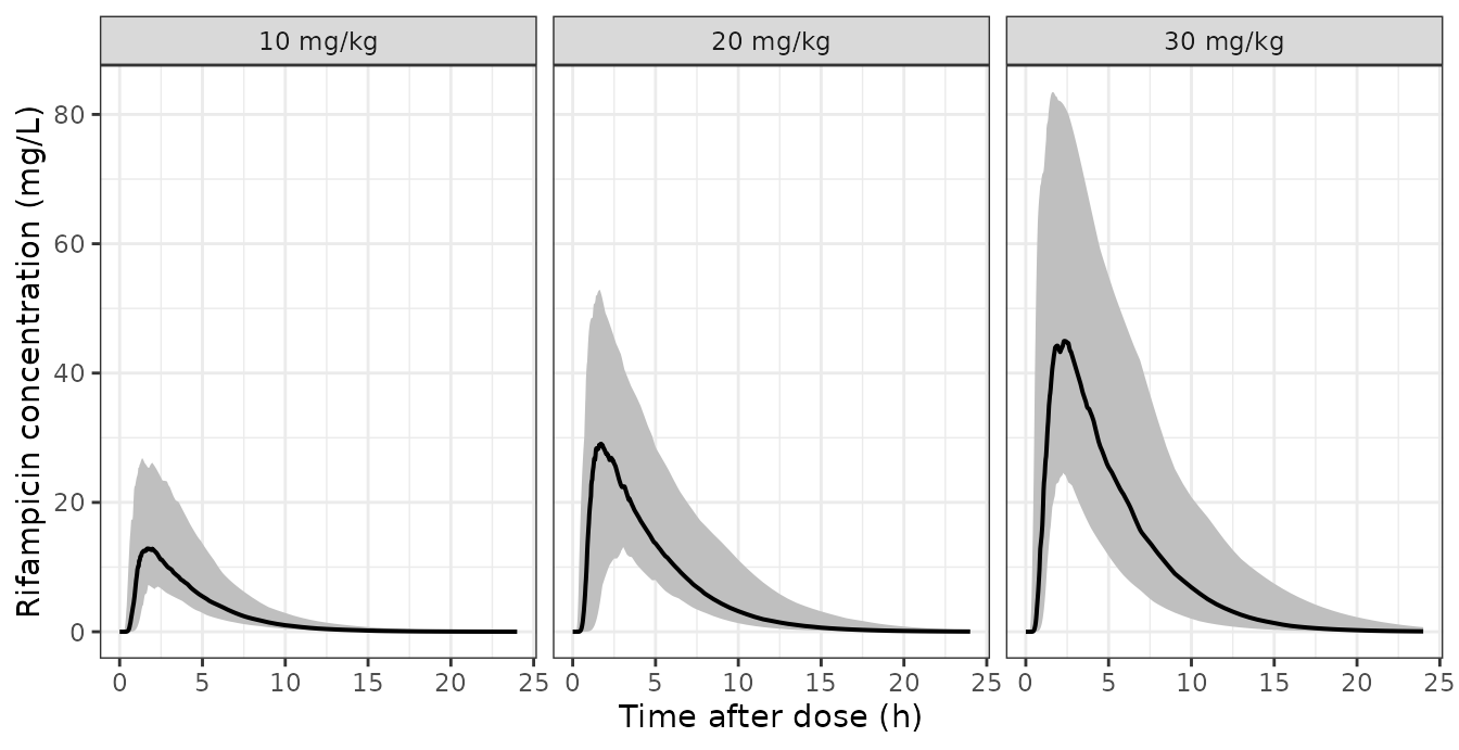
Replicates Figure 2 of Gafar 2026: simulated steady-state rifampicin concentrations by actual mg/kg dose group. Solid line is the median, shaded band the 5th-95th percentile of the simulated cohort.
Replicating Figure 3: exposure by treatment arm and country
exposure <- sim |>
  dplyr::group_by(id, country, arm, grp) |>
  dplyr::summarise(
    AUC = trapz(tad, Cc),
    Cmax = max(Cc),
    .groups = "drop"
  )
exposure |>
  tidyr::pivot_longer(c(AUC, Cmax), names_to = "metric", values_to = "value") |>
  dplyr::mutate(
    metric = factor(metric, levels = c("AUC", "Cmax"),
                    labels = c("AUC[0-24] (mg*h/L)", "Cmax (mg/L)")),
    arm = factor(paste0(arm, " mg/kg"), levels = paste0(c(10, 20, 30), " mg/kg"))
  ) |>
  ggplot(aes(arm, value, fill = country)) +
  geom_boxplot(coef = 0, outlier.shape = NA, position = position_dodge(width = 0.8)) +
  stat_summary(fun.min = function(x) stats::quantile(x, 0.025),
               fun.max = function(x) stats::quantile(x, 0.975),
               geom = "errorbar", width = 0.3,
               position = position_dodge(width = 0.8)) +
  facet_wrap(~metric, scales = "free_y") +
  labs(x = NULL, y = NULL, fill = "Country") +
  theme_bw()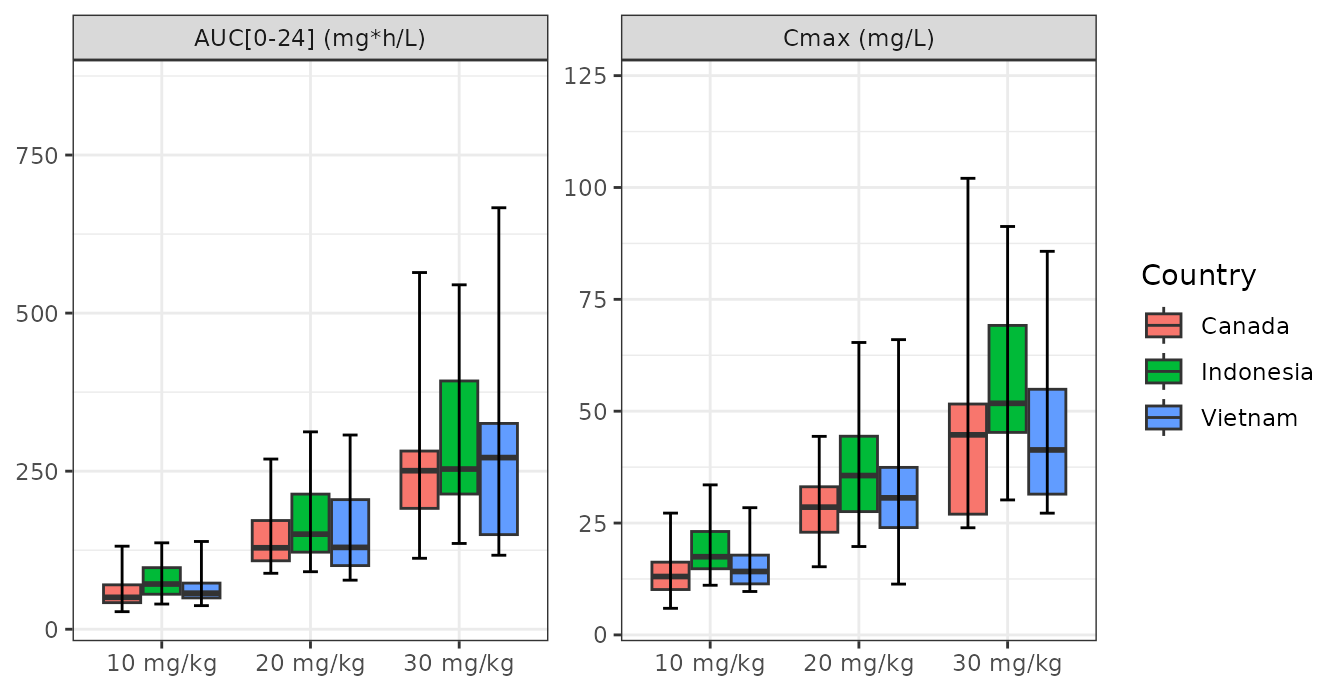
Replicates Figure 3 of Gafar 2026: model-derived AUC0-24 and Cmax by treatment arm (actual mg/kg dose) and country. Boxes are the interquartile range, the line the median, whiskers the 2.5th and 97.5th percentiles.
Typical-value replication of Table 3
Table 3 reports the median model-derived AUC0-24 and
Cmax per dose group and country. The tightest available check
is deterministic: run one typical subject
(rxode2::zeroRe(), so no random effects) per country and
arm, at that country’s median body weight, fat-free mass and
actual mg/kg dose from Table S7, and compare against
the Table 3 median.
ctry <- tibble::tribble(
  ~country,     ~WT,  ~FFM, ~ca, ~vn,
  "Canada",    73.8,  51.3,  1L,  0L,
  "Indonesia", 58.1,  40.1,  0L,  0L,
  "Vietnam",   57.0,  38.0,  0L,  1L
)
# Table S7 median actual mg/kg dose by country and arm.
mgkg_tab <- tibble::tribble(
  ~country,    ~arm, ~mgkg,
  "Canada",     10L,  9.1,   "Canada",     20L, 18.6,  "Canada",     30L, 28.7,
  "Indonesia",  10L,  9.1,   "Indonesia",  20L, 19.2,  "Indonesia",  30L, 28.1,
  "Vietnam",    10L,  9.5,   "Vietnam",    20L, 19.7,  "Vietnam",    30L, 28.6
)
# Table 3 medians.
key3 <- tibble::tribble(
  ~country,    ~arm, ~auclast, ~cmax,
  "Canada",     10L,  58.5,  14.7,  "Canada",     20L, 135.6, 29.0,  "Canada",     30L, 164.0, 35.7,
  "Indonesia",  10L,  69.5,  17.8,  "Indonesia",  20L, 176.4, 40.0,  "Indonesia",  30L, 272.5, 55.7,
  "Vietnam",    10L,  58.1,  15.5,  "Vietnam",    20L, 141.1, 32.4,  "Vietnam",    30L, 234.0, 51.7
)

typical <- mgkg_tab |>
  dplyr::left_join(ctry, by = "country") |>
  dplyr::mutate(dose = mgkg * WT)

typ_res <- lapply(seq_len(nrow(typical)), function(i) {
  g <- typical[i, ]
  s <- solve_one(dose = g$dose, FFM = g$FFM, ca = g$ca, vn = g$vn)
  tibble::tibble(country = g$country, arm = g$arm,
                 auclast = trapz(s$tad, s$Cc), cmax = max(s$Cc))
}) |>
  dplyr::bind_rows()
#> ℹ omega/sigma items treated as zero: 'etalclint_max', 'etalvc', 'etalkm', 'etaiov_fdepot_1', 'etaiov_fdepot_2', 'etaiov_ka_1', 'etaiov_ka_2', 'etaiov_mtt_1', 'etaiov_mtt_2'
#> ℹ omega/sigma items treated as zero: 'etalclint_max', 'etalvc', 'etalkm', 'etaiov_fdepot_1', 'etaiov_fdepot_2', 'etaiov_ka_1', 'etaiov_ka_2', 'etaiov_mtt_1', 'etaiov_mtt_2'
#> ℹ omega/sigma items treated as zero: 'etalclint_max', 'etalvc', 'etalkm', 'etaiov_fdepot_1', 'etaiov_fdepot_2', 'etaiov_ka_1', 'etaiov_ka_2', 'etaiov_mtt_1', 'etaiov_mtt_2'
#> ℹ omega/sigma items treated as zero: 'etalclint_max', 'etalvc', 'etalkm', 'etaiov_fdepot_1', 'etaiov_fdepot_2', 'etaiov_ka_1', 'etaiov_ka_2', 'etaiov_mtt_1', 'etaiov_mtt_2'
#> ℹ omega/sigma items treated as zero: 'etalclint_max', 'etalvc', 'etalkm', 'etaiov_fdepot_1', 'etaiov_fdepot_2', 'etaiov_ka_1', 'etaiov_ka_2', 'etaiov_mtt_1', 'etaiov_mtt_2'
#> ℹ omega/sigma items treated as zero: 'etalclint_max', 'etalvc', 'etalkm', 'etaiov_fdepot_1', 'etaiov_fdepot_2', 'etaiov_ka_1', 'etaiov_ka_2', 'etaiov_mtt_1', 'etaiov_mtt_2'
#> ℹ omega/sigma items treated as zero: 'etalclint_max', 'etalvc', 'etalkm', 'etaiov_fdepot_1', 'etaiov_fdepot_2', 'etaiov_ka_1', 'etaiov_ka_2', 'etaiov_mtt_1', 'etaiov_mtt_2'
#> ℹ omega/sigma items treated as zero: 'etalclint_max', 'etalvc', 'etalkm', 'etaiov_fdepot_1', 'etaiov_fdepot_2', 'etaiov_ka_1', 'etaiov_ka_2', 'etaiov_mtt_1', 'etaiov_mtt_2'
#> ℹ omega/sigma items treated as zero: 'etalclint_max', 'etalvc', 'etalkm', 'etaiov_fdepot_1', 'etaiov_fdepot_2', 'etaiov_ka_1', 'etaiov_ka_2', 'etaiov_mtt_1', 'etaiov_mtt_2'

cmp3 <- typ_res |>
  dplyr::rename(sim_auclast = auclast, sim_cmax = cmax) |>
  dplyr::left_join(key3, by = c("country", "arm")) |>
  dplyr::mutate(
    auc_pd = 100 * (sim_auclast - auclast) / auclast,
    cmax_pd = 100 * (sim_cmax - cmax) / cmax,
    Group = paste0(country, " ", arm, " mg/kg")
  )

cmp3 |>
  dplyr::transmute(
    Group,
    `AUC0-24 published (mg*h/L)` = auclast,
    `AUC0-24 simulated` = round(sim_auclast, 1),
    `AUC % diff` = round(auc_pd, 1),
    `Cmax published (mg/L)` = cmax,
    `Cmax simulated` = round(sim_cmax, 1),
    `Cmax % diff` = round(cmax_pd, 1)
  ) |>
  knitr::kable(
    caption = paste(
      "Typical-value (zeroRe) replication of Gafar 2026 Table 3. The Canada",
      "30 mg/kg row is not a usable reference: the source footnote a records",
      "that only n = 2 Canadian participants received the triple dose, so the",
      "Table 3 entry is a two-subject minimum-maximum range, not a cohort",
      "median."
    )
)| Group | AUC0-24 published (mg*h/L) | AUC0-24 simulated | AUC % diff | Cmax published (mg/L) | Cmax simulated | Cmax % diff |
|---|---|---|---|---|---|---|
| Canada 10 mg/kg | 58.5 | 54.0 | -7.7 | 14.7 | 13.2 | -10.5 |
| Canada 20 mg/kg | 135.6 | 124.3 | -8.3 | 29.0 | 28.0 | -3.5 |
| Canada 30 mg/kg | 164.0 | 214.6 | 30.8 | 35.7 | 44.6 | 24.9 |
| Indonesia 10 mg/kg | 69.5 | 67.6 | -2.7 | 17.8 | 17.0 | -4.7 |
| Indonesia 20 mg/kg | 176.4 | 166.2 | -5.8 | 40.0 | 37.6 | -6.0 |
| Indonesia 30 mg/kg | 272.5 | 273.8 | 0.5 | 55.7 | 56.8 | 1.9 |
| Vietnam 10 mg/kg | 58.1 | 62.7 | 7.9 | 15.5 | 16.0 | 3.2 |
| Vietnam 20 mg/kg | 141.1 | 149.9 | 6.2 | 32.4 | 34.8 | 7.3 |
| Vietnam 30 mg/kg | 234.0 | 242.8 | 3.8 | 51.7 | 52.0 | 0.6 |
powered <- dplyr::filter(cmp3, !(country == "Canada" & arm == 30L))

stopifnot(
  # Deterministic (zeroRe), so no cross-version sampling noise: assert on the
  # centre and on the whole set of adequately powered cells.
  abs(stats::median(powered$auc_pd)) < 5,
  max(abs(powered$auc_pd)) < 10,
  abs(stats::median(powered$cmax_pd)) < 5,
  max(abs(powered$cmax_pd)) < 12,
  # Ordering claim from Results: exposure is highest in Indonesia, then
  # Vietnam, then Canada, at every dose level.
  all(
    dplyr::filter(typ_res, country == "Indonesia")$auclast >
      dplyr::filter(typ_res, country == "Vietnam")$auclast
  ),
  all(
    dplyr::filter(typ_res, country == "Vietnam")$auclast >
      dplyr::filter(typ_res, country == "Canada")$auclast
  )
)
The eight adequately powered cells reproduce the published medians with a median absolute difference of 6.0% on AUC0-24 and 4.1% on Cmax, from a single typical subject compared against a cohort median. The Canada 30 mg/kg cell is excluded on the source paper’s own authority.
PKNCA validation
sim_nca <- sim |>
  dplyr::filter(!is.na(Cc)) |>
  dplyr::select(id, tad, Cc, grp)

# Defensive time-zero row (rifampicin is given orally, so pre-dose Cc = 0 is
# the correct value if the grid did not already supply t = 0).
sim_nca <- dplyr::bind_rows(
  sim_nca,
  sim_nca |>
    dplyr::distinct(id, grp) |>
    dplyr::mutate(tad = 0, Cc = 0)
) |>
  dplyr::arrange(id, tad) |>
  dplyr::distinct(id, tad, .keep_all = TRUE)

dose_df <- cohort |>
  dplyr::transmute(id, grp, tad = 0, amt = dose)

conc_obj <- PKNCA::PKNCAconc(sim_nca, Cc ~ tad | grp + id,
                             concu = "mg/L", timeu = "h")
dose_obj <- PKNCA::PKNCAdose(dose_df, amt ~ tad | grp + id, doseu = "mg")

intervals <- data.frame(
  start = 0, end = 24,
  cmax = TRUE, tmax = TRUE, auclast = TRUE, half.life = TRUE
)

nca <- PKNCA::pk.nca(PKNCA::PKNCAdata(conc_obj, dose_obj, intervals = intervals))
ref_nca <- key3 |>
  dplyr::transmute(grp = paste0(country, " ", arm, " mg/kg"), auclast, cmax)

tbl <- nlmixr2lib::ncaComparisonTable(
  simulated = nca,
  reference = ref_nca,
  by = "grp",
  params = c("cmax", "auclast"),
  units = c(cmax = "mg/L", auclast = "mg*h/L")
)

tbl |>
  dplyr::rename(Group = grp) |>
  knitr::kable(
    caption = paste(
      "PKNCA steady-state (0-24 h) exposure from the simulated cohort against",
      "the Gafar 2026 Table 3 medians. Rows differing by more than 20% are",
      "starred. The Canada 30 mg/kg reference is a two-subject",
      "minimum-maximum range (source Table 3 footnote a), not a cohort median."
    )
)| NCA parameter | Group | Reference | Simulated | % diff |
|---|---|---|---|---|
| Cmax (mg/L) | Canada 10 mg/kg | 14.7 | 11.8 | -19.5% |
| Cmax (mg/L) | Canada 20 mg/kg | 29 | 27 | -7.0% |
| Cmax (mg/L) | Canada 30 mg/kg | 35.7 | 41.6 | +16.6% |
| Cmax (mg/L) | Indonesia 10 mg/kg | 17.8 | 17.7 | -0.6% |
| Cmax (mg/L) | Indonesia 20 mg/kg | 40 | 35.9 | -10.3% |
| Cmax (mg/L) | Indonesia 30 mg/kg | 55.7 | 59.3 | +6.5% |
| Cmax (mg/L) | Vietnam 10 mg/kg | 15.5 | 15.8 | +2.1% |
| Cmax (mg/L) | Vietnam 20 mg/kg | 32.4 | 29.3 | -9.7% |
| Cmax (mg/L) | Vietnam 30 mg/kg | 51.7 | 47.5 | -8.0% |
| AUClast (mg*h/L) | Canada 10 mg/kg | 58.5 | 57.8 | -1.2% |
| AUClast (mg*h/L) | Canada 20 mg/kg | 136 | 135 | -0.1% |
| AUClast (mg*h/L) | Canada 30 mg/kg | 164 | 193 | +17.9% |
| AUClast (mg*h/L) | Indonesia 10 mg/kg | 69.5 | 76.4 | +9.9% |
| AUClast (mg*h/L) | Indonesia 20 mg/kg | 176 | 197 | +11.6% |
| AUClast (mg*h/L) | Indonesia 30 mg/kg | 272 | 287 | +5.3% |
| AUClast (mg*h/L) | Vietnam 10 mg/kg | 58.1 | 61.9 | +6.6% |
| AUClast (mg*h/L) | Vietnam 20 mg/kg | 141 | 125 | -11.5% |
| AUClast (mg*h/L) | Vietnam 30 mg/kg | 234 | 223 | -4.6% |
attr(tbl, "footnote")
#> NULL
nca_res <- as.data.frame(nca$result) |>
  dplyr::filter(PPTESTCD %in% c("cmax", "auclast")) |>
  dplyr::group_by(grp, PPTESTCD) |>
  dplyr::summarise(sim = stats::median(PPORRES, na.rm = TRUE), .groups = "drop") |>
  tidyr::pivot_wider(names_from = PPTESTCD, values_from = sim) |>
  dplyr::left_join(ref_nca, by = "grp", suffix = c("_sim", "_ref")) |>
  dplyr::filter(grp != "Canada 30 mg/kg") |>
  dplyr::mutate(
    auc_pd = 100 * (auclast_sim - auclast_ref) / auclast_ref,
    cmax_pd = 100 * (cmax_sim - cmax_ref) / cmax_ref
  )

stopifnot(
  # A NaN here would make every comparison below vacuously NA rather than
  # failing, so check the medians are finite before checking their size.
  all(is.finite(nca_res$auc_pd)), all(is.finite(nca_res$cmax_pd)),
  # Monte-Carlo cohort medians: assert on the centre and on a robust envelope,
  # never on the extreme cell. The covariate draw and the eta draw -- not the
  # model -- decide where the tails land, and rxode2's random stream is not
  # stable across versions, so a max() bound here would be a CI coin flip.
  # The tight, reproducible check on this transcription is the deterministic
  # zeroRe comparison above (median < 5%, worst cell < 10%).
  abs(stats::median(nca_res$auc_pd)) < 15,
  stats::quantile(abs(nca_res$auc_pd), 0.9) < 30,
  abs(stats::median(nca_res$cmax_pd)) < 15,
  stats::quantile(abs(nca_res$cmax_pd), 0.9) < 30
)
Dose proportionality (Table S5)
Table S5 reports the percentage increase in median steady-state exposure at 20 and 30 mg/kg relative to 10 mg/kg, from 1000 simulated trials. The deterministic typical-value run reproduces the same pattern.
prop_tab <- typ_res |>
  dplyr::select(country, arm, auclast, cmax) |>
  tidyr::pivot_longer(c(auclast, cmax), names_to = "metric") |>
  dplyr::group_by(country, metric) |>
  dplyr::mutate(pct = 100 * (value / value[arm == 10L] - 1)) |>
  dplyr::ungroup() |>
  dplyr::filter(arm != 10L)

key_s5 <- tibble::tribble(
  ~country,     ~arm, ~metric,   ~published,
  "Canada",     20L, "auclast", 125,   "Canada",     30L, "auclast", 202,
  "Indonesia",  20L, "auclast", 149,   "Indonesia",  30L, "auclast", 276,
  "Vietnam",    20L, "auclast", 128,   "Vietnam",    30L, "auclast", 296,
  "Canada",     20L, "cmax",    102,   "Canada",     30L, "cmax",    146,
  "Indonesia",  20L, "cmax",    126,   "Indonesia",  30L, "cmax",    216,
  "Vietnam",    20L, "cmax",    113,   "Vietnam",    30L, "cmax",    240
)

prop_tab |>
  dplyr::left_join(key_s5, by = c("country", "arm", "metric")) |>
  dplyr::transmute(
    Country = country,
    Comparison = paste0(arm, " vs 10 mg/kg"),
    Metric = ifelse(metric == "auclast", "AUC0-24", "Cmax"),
    `Published increase (%)` = published,
    `Simulated increase (%)` = round(pct)
  ) |>
  knitr::kable(
    caption = paste(
      "Replicates Gafar 2026 Table S5. The published values are medians over",
      "1000 clinical trial simulations that resampled participant covariates",
      "from the modelling dataset and used the protocol weight-band doses;",
      "the simulated column is one typical subject per country at the Table S7",
      "median actual mg/kg dose, so the two arms of each comparison differ",
      "slightly in dose ratio. The Canada 30 mg/kg arm rests on n = 2."
    )
)| Country | Comparison | Metric | Published increase (%) | Simulated increase (%) |
|---|---|---|---|---|
| Canada | 20 vs 10 mg/kg | AUC0-24 | 125 | 130 |
| Canada | 20 vs 10 mg/kg | Cmax | 102 | 113 |
| Canada | 30 vs 10 mg/kg | AUC0-24 | 202 | 297 |
| Canada | 30 vs 10 mg/kg | Cmax | 146 | 239 |
| Indonesia | 20 vs 10 mg/kg | AUC0-24 | 149 | 146 |
| Indonesia | 20 vs 10 mg/kg | Cmax | 126 | 122 |
| Indonesia | 30 vs 10 mg/kg | AUC0-24 | 276 | 305 |
| Indonesia | 30 vs 10 mg/kg | Cmax | 216 | 235 |
| Vietnam | 20 vs 10 mg/kg | AUC0-24 | 128 | 139 |
| Vietnam | 20 vs 10 mg/kg | Cmax | 113 | 117 |
| Vietnam | 30 vs 10 mg/kg | AUC0-24 | 296 | 287 |
| Vietnam | 30 vs 10 mg/kg | Cmax | 240 | 225 |
stopifnot(
  # The paper's headline claim is greater-than-proportional accumulation of
  # exposure, so assert the inequality rather than the exact percentage.
  all(dplyr::filter(prop_tab, arm == 20L, metric == "auclast")$pct > 100),
  all(dplyr::filter(prop_tab, arm == 30L, metric == "auclast")$pct > 200)
)
Assumptions and deviations
Erratum: the residual-error rows of Table 2 are
back-transformed with a formula that does not apply to them.
Table 2 prints the two proportional residual errors as 35.1 CV% (sparse
sampling) and 45.3 CV% (intensive sampling). The published NONMEM
control stream (Supplementary Appendix 1) sets
PROP = IPRED*THETA(13),
IF(ITS.EQ.1) PROP = IPRED*THETA(14),
SD = SQRT(ADD**2 + PROP**2),
Y = IPRED + SD*ERR(1) with $SIGMA 1 FIX, and
$THETA (0, 0.116) and (0, 0.187). Those thetas
are therefore linear proportional standard deviations -
11.6% and 18.7%. Applying the Table 2 footnote-a formula for the OMEGA
rows,
, to them gives 35.07% and
45.35%, reproducing the printed 35.1 and 45.3 to three significant
figures. Two independent exact matches make it clear that the table’s
residual-error CV% column was generated by applying the log-normal OMEGA
transformation to a linear proportional-error coefficient, which
overstates the residual error roughly threefold. Following the standing
rule that a deposited control stream beats a back-transformed table,
this model uses 0.116 and 0.187. Every other Table 2 row agrees exactly
with its $THETA / $OMEGA counterpart, which is
what makes the residual rows identifiable as the exception rather than
as a stale set of initial estimates.
Between-subject variability on Km enters multiplicatively on
the log scale. The control stream codes
LOGKM = THETA(10)*EXP(IIVKM) and then uses
EXP(LOGKM) wherever
is required, so the random effect scales the logarithm of
rather than being added to it. The model file reproduces this literally
(km <- exp(lkm * exp(etalkm))). It is unusual, and it
means the “14.7 CV%” of Table 2 is the coefficient of variation of the
multiplier on
,
not of
:
a one-standard-deviation draw moves
from 64.1 mg/L to about 36 or 123 mg/L.
Between-occasion variability is expanded into per-occasion
etas. rxode2 parses the eta ~ var | occ
multi-level syntax but cannot simulate from it, so the
$OMEGA BLOCK(1) <value> +
$OMEGA BLOCK(1) SAME pairs are written out as
etaiov_*_1 (estimated) and etaiov_*_2
(fix()ed to the same variance), multiplexed by the
canonical OCC column. This is also the more faithful
translation, since it is exactly what the $PK block’s
IF (OCC.EQ.1) THEN ... ELSE ... construct does. Pass
OCC = 1 for a single-occasion simulation. The model emits a
some etas defaulted to non-mu referenced warning from this
idiom; it affects estimation only, not simulation, and is the accepted
cost of the pattern (Jonsson_2011_ethambutol.R emits the
same warning).
Country versus formulation. Country and rifampicin
product are completely confounded in 2R2, and the control stream’s
driver column is FRM (formulation), not country. The effect
is registered here as REGION_CANADA /
REGION_VIETNAM because the retained model pools Vietnam’s
two formulations into a single indicator (fitting them separately gave a
1-point OFV change over 3 extra parameters), so what is identified is a
country-level contrast and the formulation attribution is the authors’
interpretation. covariateData records the FRM
coding for anyone building a dataset against the source.
The IF (CH>0) guard in $DES is
not reproduced. The control stream sets SAT_CL = 0
when the liver concentration is zero. Every term that
SAT_CL feeds is multiplied by the liver amount, which is
also zero at that instant, so the branch is provably a no-op; the smooth
form is used here so the solver sees no discontinuity.
Below-the-limit-of-quantification handling is not
reproduced. The $ERROR block inflates the additive
error by LLOD/2 for imputed censored records
(IF(ICALL.EQ.2.AND.BLQ.EQ.1)) and sets an effectively
infinite SD for the M3-style records (BLQ.EQ.2). Both are
estimation-time constructs for Beal-M6 censoring and have no meaning in
forward simulation, so the model carries the uninflated
addSd = 0.025 mg/L.
No AUC accumulator compartment. The control stream
carries a fourth compartment, DADT(4) = A(3)/V, purely to
report AUC, plus COM(1)/COM(2) bookkeeping for
Cmax and Tmax. These are output conveniences with no feedback into the
system; AUC and Cmax are computed here with PKNCA instead.
Table 3 is post-hoc, the simulated cohort is a fresh draw. The published AUC0-24 and Cmax values are model-derived individual predictions - empirical Bayes estimates conditioned on each participant’s own observations - whereas the virtual cohort draws random effects afresh. With between-subject CVs of only 11.7-14.9% the two medians are close, but they are not the same quantity.
Cohort construction assumptions the paper does not specify. Body weight is drawn log-normal from the per-country median and IQR of Table S7 and body mass index from the cohort median and IQR of Table 1, independently; the paper reports no joint distribution. Sex is drawn at the pooled 57.9% female rate because Table S7 does not break sex down by country. Doses follow the Table S3 weight bands applied to the drawn weight, which is why the simulated actual mg/kg distribution is wider than a single target dose.
Autoinduction is absent by design. The reference model of Chirehwa 2016 includes rifampicin autoinduction; Gafar 2026 dropped it because sampling was performed once, at week 4, when autoinduction is complete. The model therefore describes week-4 steady state and must not be used to simulate the first weeks of treatment.