Nirmatrelvir/ritonavir in critically ill adults (Chen 2024)

Model and source

Chen 2024 fit two independent one-compartment models to the same 89 plasma samples from 31 critically ill adults: one for ritonavir and one for nirmatrelvir. They are separate fits with separate objective functions (Tables 2 and 3), so they are packaged as two model files, and this single vignette walks the paper as a unit.

The two models are not merely parallel: the nirmatrelvir clearance model takes the ritonavir 12 h dosing-interval AUC as a covariate, and the paper’s Equation 2 defines that covariate as AUC = DOSE / (CL/F) computed from the ritonavir fit. So the ritonavir model supplies a covariate column to the nirmatrelvir model, and the two compose directly. That composition is exercised throughout this vignette.

• Ritonavir citation: Chen N, Yu X, Li L, Yang P, Dong R, Huang Y, Ling X, Shentu Q, Yu W, Jiang S. Target Attainment and Population Pharmacokinetics of Nirmatrelvir/Ritonavir in Critically Ill Adult Patients. Infect Drug Resist. 2024;17:4055-4065. doi:10.2147/IDR.S471918
• Nirmatrelvir description: One-compartment first-order-absorption population PK model for oral nirmatrelvir given as the nirmatrelvir/ritonavir fixed combination in critically ill adults with COVID-19; apparent clearance depends on CKD-EPI creatinine clearance and on the co-administered ritonavir 12 h dosing-interval AUC through a doubly-centred power function, with correlated interindividual variability on CL/F and V/F (Chen 2024).
• Article: https://doi.org/10.2147/IDR.S471918 (open access; PMCID PMC11416114)

No data supplement accompanies the article. The EuropePMC supplementary-file bundle for PMC11416114 contains only the publisher’s figure and equation images; Equations 1 and 2 were read from those equation images (IDR-17-4055-e0001, IDR-17-4055-e0002) because both are vector graphics that no text extraction of the PDF recovers.

Population

Thirty-one adults admitted to the intensive care unit of the First Affiliated Hospital of Zhejiang University School of Medicine between January and June 2023 with RT-PCR-confirmed SARS-CoV-2 infection and compatible pulmonary CT findings (Table 1). Median age 69 years (IQR 63-77), 65% male, mean body weight 60.6 kg (SD 12.8). Median APACHE II score 14 (IQR 11-21) and median SOFA score 6 (IQR 3-9). Creatinine clearance by the CKD-EPI equation was 78.5 +/- 34.4 mL/min. Patients on continuous renal replacement therapy or ECMO were excluded.

Nirmatrelvir/ritonavir was given as 300 mg/100 mg twice daily to 27 patients (87%) and 150 mg/100 mg twice daily to 4 (13%); the ritonavir component was 100 mg twice daily in every patient. Twenty-nine patients (94%) received the tablets by nasal feeding and 2 (6%) orally, all for more than five days. Two to three serial plasma samples per patient were drawn after the second dose.

The same information is available programmatically via each model’s population metadata (rxode2::rxode(readModelDb("Chen_2024_nirmatrelvir"))$population).

Source trace

Equation / parameter	Value	Source location
Ritonavir structural model: 1-compartment, first-order absorption	n/a	Results, Population PK Model Development (one- vs two-compartment OFV 193.6 vs 193.2)
lka (ritonavir)	0.64 1/h	Table 2, tvKa (RSE 37.4%)
lvc (ritonavir)	84.9 L	Table 2, tvV (RSE 29.2%)
lcl (ritonavir)	10.3 L/h	Table 2, tvCL (RSE 14.7%)
etalcl + etalvc block (ritonavir)	0.57, 0.621, 1.27	Table 2: omega^2 CL 0.57, omega^2 V 1.27, CorrV-CL 0.73; covariance = 0.73 * sqrt(0.57 * 1.27)
expSd (ritonavir)	0.34	Table 2, Stdev0 (RSE 12.7%); “log-additive error option” per Results
Nirmatrelvir structural model: 1-compartment, first-order absorption	n/a	Results (one- vs two-compartment OFV 125.5 vs 125.7)
lka (nirmatrelvir)	0.42 1/h	Table 3, tvKa (RSE 24.9%)
lvc (nirmatrelvir)	36.5 L	Table 3, tvV (RSE 23.3%)
lcl (nirmatrelvir)	3.6 L/h	Table 3, tvCL (RSE 7.1%)
e_crcl_cl	0.53	Table 3, dCLdCrCL (RSE 21.7%)
e_rtv_auc_12h_cl	-0.45	Table 3, dCLdAUCRIT (RSE magnitude 18.0%)
CL/F covariate equation	CL = tvCL * (CrCL/80)^dCLdCrCL * (AUCRIT/12.2)^dCLdRIT * exp(nCL)	Equation 1 (publisher equation image IDR-17-4055-e0001); the centring constants 80 and 12.2 appear only here
AUCRIT definition	AUC = DOSE / (CL/F), DOSE = 100 mg	Equation 2 (IDR-17-4055-e0002); Figure 1 caption (“AUC, area under curve of ritonavir base on 100mg”)
etalcl + etalvc block (nirmatrelvir)	0.086, 0.02815, 0.64	Table 3: omega^2 CL 0.086, omega^2 V 0.64, CorrV-CL 0.12; covariance = 0.12 * sqrt(0.086 * 0.64)
expSd (nirmatrelvir)	0.26	Table 3, stdev (RSE 17.4%)
Total EC90 target	292 ng/mL = 0.292 mg/L	Discussion (“With approximately 70% protein binding, the total EC90 for NIR is 292 ng/mL”) and Monte Carlo Dosing Simulations
Free EC90	90.5 ng/mL (181 nM)	Discussion
Human NOAEL ceiling	79,700 ng/mL = 79.7 mg/L	Monte Carlo Dosing Simulations
AUCRIT simulation range (10th-90th percentile)	3.2 to 23.3 mg*h/L	Monte Carlo Dosing Simulations; Table 4 column breakpoints
Bayesian-feedback AUC, nirmatrelvir 300 mg	107.1 ugh/mL = 107.1 mgh/L	Discussion paragraph 2
Median steady-state Ctrough vs total EC90	> 5.7-fold	Discussion, final paragraph

CV, % in Tables 2 and 3 is the relative standard error of the estimate, not interindividual variability. The Abstract reports the nirmatrelvir parameters as “Mean (SD) … 0.42 (0.10) h-1, 36.5 (8.5) L, 3.6 (0.26) L/h”, which are exactly the Table 3 estimates multiplied by the Table 3 CV, % values (0.42 x 24.9% = 0.105; 36.5 x 23.3% = 8.5; 3.6 x 7.1% = 0.256). Interindividual variability is reported separately as omega^2.

EC90_TOTAL <- 0.292    # mg/L; total EC90 for SARS-CoV-2 (Discussion)
NOAEL      <- 79.7     # mg/L; human no-observed-adverse-effect level
RIT_DOSE   <- 100      # mg; ritonavir dose in every regimen
TAU        <- 12       # h; q12h dosing interval
DOSE_TIMES <- seq(0, 108, by = TAU)   # 10 doses = 5 days of q12h therapy
SS_START   <- max(DOSE_TIMES)         # start of the final (steady-state) interval
SS_END     <- SS_START + TAU

nir <- readModelDb("Chen_2024_nirmatrelvir")
rit <- readModelDb("Chen_2024_ritonavir")

Structural check: the centring constants and the closed form

Before simulating a cohort, verify against the analytic one-compartment oral steady-state solution. Setting CRCL = 80 and CONMED_RTV_AUC_12h = 12.2 makes both covariate factors of Equation 1 exactly 1, so the model must return cl = 3.6 L/h – the Table 3 typical value. This is a direct test that the two centring constants, which appear nowhere except inside Equation 1, were transcribed correctly: mistyping either one changes cl immediately.

Both sides of this comparison use the same parameters, so the only difference is ODE-solver numerical error and a tight bound is the correct gate here.

ev_typ <- rxode2::et(amt = 300, cmt = "depot", time = DOSE_TIMES) |>
  rxode2::et(seq(0, 120, by = 0.25), cmt = "central") |>
  as.data.frame() |>
  dplyr::mutate(id = 1L, CRCL = 80, CONMED_RTV_AUC_12h = 12.2)

sim_typ <- rxode2::rxSolve(rxode2::zeroRe(nir), events = ev_typ) |>
  as.data.frame()
#> ℹ parameter labels from comments will be replaced by 'label()'
#> ℹ omega/sigma items treated as zero: 'etalcl', 'etalvc'

cl_typ <- unique(round(sim_typ$cl, 10))
vc_typ <- unique(round(sim_typ$vc, 10))
ka_typ <- unique(round(sim_typ$ka, 10))
stopifnot(length(cl_typ) == 1L, length(vc_typ) == 1L, length(ka_typ) == 1L)

# Both covariate factors are exactly 1 at the centring point, so cl must be the
# Table 3 typical value 3.6 L/h and vc the Table 3 value 36.5 L.
stopifnot(
  abs(cl_typ - 3.6)  < 1e-8,
  abs(vc_typ - 36.5) < 1e-8,
  abs(ka_typ - 0.42) < 1e-8
)

kel_typ <- cl_typ / vc_typ

# Analytic one-compartment, first-order absorption, steady-state concentration
# at time t after a dose in the interval (Gibaldi & Perrier superposition).
css_oral <- function(t, dose, ka, kel, vc, tau) {
  (dose * ka / (vc * (ka - kel))) *
    (exp(-kel * t) / (1 - exp(-kel * tau)) -
       exp(-ka  * t) / (1 - exp(-ka  * tau)))
}

ss <- sim_typ |>
  dplyr::filter(time >= SS_START, time <= SS_END) |>
  dplyr::mutate(
    t_in_interval = time - SS_START,
    Cc_closed = css_oral(t_in_interval, 300, ka_typ, kel_typ, vc_typ, TAU)
  )

rel_err <- abs(ss$Cc / ss$Cc_closed - 1)
max_rel_err <- max(rel_err)

# 1e-4 is far above the observed solver error but far below any transcription
# error: a wrong ka, V or dose moves this by orders of magnitude.
stopifnot(max_rel_err < 1e-4)

ctrough_typ <- ss$Cc[ss$t_in_interval == TAU]
cmax_typ    <- max(ss$Cc)

tibble::tibble(
  Quantity = c("Typical CL/F (L/h)", "Typical V/F (L)", "Typical ka (1/h)",
               "Steady-state Cmax (mg/L)", "Steady-state Ctrough (mg/L)",
               "Steady-state Ctrough / total EC90",
               "Max |solved / closed-form - 1| over the interval"),
  Value = c(cl_typ, vc_typ, ka_typ, cmax_typ, ctrough_typ,
            ctrough_typ / EC90_TOTAL, max_rel_err)
) |>
  knitr::kable(digits = 6,
               caption = "Typical-value structural check, nirmatrelvir 300 mg q12h at the covariate centring point.")

Typical-value structural check, nirmatrelvir 300 mg q12h at the covariate centring point.

Quantity	Value
Typical CL/F (L/h)	3.600000
Typical V/F (L)	36.500000
Typical ka (1/h)	0.420000
Steady-state Cmax (mg/L)	8.476520
Steady-state Ctrough (mg/L)	4.670378
Steady-state Ctrough / total EC90	15.994444
Max |solved / closed-form - 1| over the interval	0.000024

The typical steady-state peak stays far below the 79.7 mg/L NOAEL ceiling the paper imposes on its simulations.

stopifnot(cmax_typ < NOAEL)

Virtual cohort

Original observed data are not publicly available. The cohort below reproduces the Table 1 creatinine-clearance distribution (mean 78.5, SD 34.4 mL/min), truncated to the 15-160 mL/min range spanned by the paper’s dosing simulations.

# set.seed() seeds R's RNG, which is what draws the CRCL column below. It does
# NOT seed rxode2's simulation RNG, and rxode2's streams are partitioned per
# solver thread -- so the eta draws differ between a 16-thread workstation and a
# 2-core CI runner. Every assertion below is written to hold for any cohort the
# model can produce (see known-vignette-failure-patterns.md pattern 12).
set.seed(20240918)
rxode2::rxSetSeed(20240918)

N_ARM <- 200L

draw_crcl <- function(n, lo = 15, hi = 160) {
  out <- numeric(0)
  while (length(out) < n) {
    x <- rnorm(2 * n, mean = 78.5, sd = 34.4)
    out <- c(out, x[x >= lo & x <= hi])
  }
  out[seq_len(n)]
}

base_subj <- tibble(
  id   = seq_len(N_ARM),
  CRCL = draw_crcl(N_ARM)
)

summary(base_subj$CRCL)
#>    Min. 1st Qu.  Median    Mean 3rd Qu.    Max. 
#>   18.08   62.17   80.61   83.02  104.21  159.55

Deriving the ritonavir-AUC covariate from the ritonavir model

Chen 2024 Equation 2 defines the nirmatrelvir covariate as AUC = DOSE / (CL/F) with DOSE = 100 mg, using each subject’s ritonavir apparent clearance. Solving the packaged ritonavir model returns per-subject cl, so the covariate column is produced by the companion model rather than invented here.

rit_events <- base_subj |>
  tidyr::crossing(time = DOSE_TIMES) |>
  dplyr::mutate(amt = RIT_DOSE, evid = 1L, cmt = "depot") |>
  dplyr::bind_rows(
    base_subj |>
      tidyr::crossing(time = seq(0, 120, by = 0.25)) |>
      dplyr::mutate(amt = NA_real_, evid = 0L, cmt = "central")
  ) |>
  dplyr::arrange(id, time, dplyr::desc(evid))

stopifnot(!anyDuplicated(unique(rit_events[, c("id", "time", "evid")])))

rit_sim <- rxode2::rxSolve(rit, events = rit_events, keep = "CRCL") |>
  as.data.frame()
#> ℹ parameter labels from comments will be replaced by 'label()'

# One CL/F per subject; AUC over the 12 h interval = 100 mg / (CL/F).
rit_cl <- rit_sim |>
  dplyr::group_by(id) |>
  dplyr::summarise(cl_rit = dplyr::first(cl), .groups = "drop") |>
  dplyr::mutate(CONMED_RTV_AUC_12h = RIT_DOSE / cl_rit)

stopifnot(nrow(rit_cl) == N_ARM, all(is.finite(rit_cl$CONMED_RTV_AUC_12h)))

auc_q <- quantile(rit_cl$CONMED_RTV_AUC_12h, c(0.10, 0.50, 0.90))
auc_q
#>       10%       50%       90% 
#>  3.728001  8.475159 20.052442

The paper swept “AUCRIT from 10%th to 90%th” in its Monte Carlo simulations, and the Table 4 dose-recommendation grid runs from 3.2 to 23.3 mg*h/L – those are the paper’s own 10th and 90th percentiles of this covariate. The ritonavir model, simulated independently, must reproduce that range: with a typical CL/F of 10.3 L/h and omega^2 CL = 0.57, the analytic 10th and 90th percentiles are 100 / (10.3 * exp(+/-1.2816 * sqrt(0.57))) = 3.7 and 25.5 mg*h/L.

This is a genuine cross-table check. It uses only Table 2 (ritonavir) to predict a range stated in the Table 4 caption and the Methods, so a mis-transcribed ritonavir CL/F or omega breaks it.

# Bounds are set wide enough to absorb the sampling spread of a 200-subject
# percentile estimate across solver-thread counts (the 10th percentile of 200
# lognormal draws with sd_log = 0.755 moves by roughly +/-20% run to run), but
# tight enough that a 2-fold error in ritonavir CL/F or a variance-vs-SD mix-up
# on omega^2 breaks them immediately.
stopifnot(
  auc_q[["10%"]] > 2.0, auc_q[["10%"]] < 6.5,
  auc_q[["90%"]] > 15.0, auc_q[["90%"]] < 40.0
)

# The Equation 1 centring constant of 12.2 mg*h/L should sit inside the
# simulated distribution, between its median and its 90th percentile: the
# median of 100/CL is 100/10.3 = 9.7 and the mean is 9.7 * exp(0.57/2) = 12.9,
# so a centring constant of 12.2 is consistent with an arithmetic-mean summary
# of this same distribution.
stopifnot(auc_q[["50%"]] < 12.2, auc_q[["90%"]] > 12.2)

Simulation: nirmatrelvir 300 mg/100 mg twice daily

nir_subj <- base_subj |>
  dplyr::left_join(rit_cl |> dplyr::select(id, CONMED_RTV_AUC_12h), by = "id")

stopifnot(nrow(nir_subj) == N_ARM, !anyNA(nir_subj$CONMED_RTV_AUC_12h))

nir_events <- nir_subj |>
  tidyr::crossing(time = DOSE_TIMES) |>
  dplyr::mutate(amt = 300, evid = 1L, cmt = "depot") |>
  dplyr::bind_rows(
    nir_subj |>
      tidyr::crossing(time = seq(0, 120, by = 0.25)) |>
      dplyr::mutate(amt = NA_real_, evid = 0L, cmt = "central")
  ) |>
  dplyr::arrange(id, time, dplyr::desc(evid))

stopifnot(!anyDuplicated(unique(nir_events[, c("id", "time", "evid")])))

nir_sim <- rxode2::rxSolve(
  nir, events = nir_events,
  keep = c("CRCL", "CONMED_RTV_AUC_12h")
) |>
  as.data.frame()
#> ℹ parameter labels from comments will be replaced by 'label()'

stopifnot(all(nir_sim$Cc >= 0))

Replicating Figure 4 (prediction-corrected VPC)

Figure 4 of Chen 2024 is a prediction-corrected VPC for each drug. The panels below show the simulated median and 5th-95th percentile envelope for both models over the five-day course, on the same axes.

vpc <- dplyr::bind_rows(
  nir_sim |>
    dplyr::transmute(time, Cc, drug = "Nirmatrelvir 300 mg q12h"),
  rit_sim |>
    dplyr::transmute(time, Cc, drug = "Ritonavir 100 mg q12h")
) |>
  dplyr::group_by(drug, time) |>
  dplyr::summarise(
    Q05 = quantile(Cc, 0.05),
    Q50 = quantile(Cc, 0.50),
    Q95 = quantile(Cc, 0.95),
    .groups = "drop"
  )

ggplot(vpc, aes(time, Q50)) +
  geom_ribbon(aes(ymin = Q05, ymax = Q95), alpha = 0.25) +
  geom_line() +
  geom_hline(
    data = data.frame(drug = "Nirmatrelvir 300 mg q12h", y = EC90_TOTAL),
    aes(yintercept = y), linetype = "dashed", colour = "firebrick"
  ) +
  facet_wrap(~drug, scales = "free_y") +
  scale_y_log10() +
  labs(
    x = "Time (h)", y = "Plasma concentration (mg/L)",
    title = "Simulated concentration-time profiles, 5 days of q12h therapy",
    caption = paste(
      "Median with 5th-95th percentile envelope, 200 virtual subjects.",
      "Companion to Figure 4 of Chen 2024. Dashed line: total EC90 =",
      EC90_TOTAL, "mg/L."
    )
  )
#> Warning in scale_y_log10(): log-10 transformation introduced infinite values.
#> log-10 transformation introduced infinite values.
#> log-10 transformation introduced infinite values.
#> log-10 transformation introduced infinite values.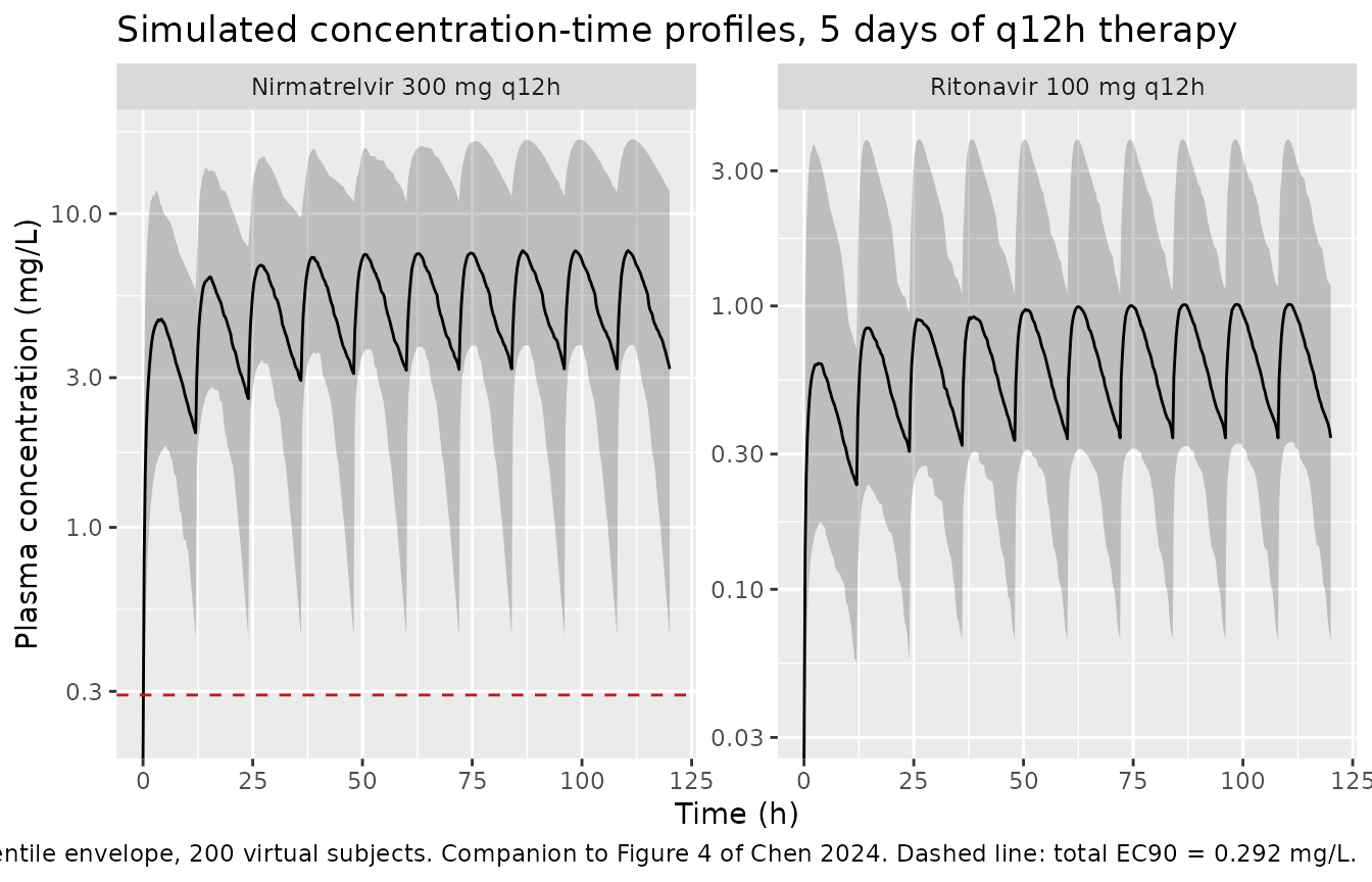

Replicating Figure 1 (CL/F versus its covariates)

Figure 1 of Chen 2024 plots individual nirmatrelvir CL/F against CrCL (panel A) and against the ritonavir AUC (panel B). Panel A is increasing and panel B decreasing, matching the signs of e_crcl_cl (+0.53) and e_rtv_auc_12h_cl (-0.45).

cl_subj <- nir_sim |>
  dplyr::group_by(id) |>
  dplyr::summarise(
    cl = dplyr::first(cl), CRCL = dplyr::first(CRCL),
    AUC_RIT = dplyr::first(CONMED_RTV_AUC_12h), .groups = "drop"
  )

cl_subj |>
  tidyr::pivot_longer(c(CRCL, AUC_RIT), names_to = "covariate", values_to = "value") |>
  dplyr::mutate(covariate = dplyr::recode(
    covariate,
    CRCL = "A: CrCL (mL/min/1.73 m^2)",
    AUC_RIT = "B: ritonavir AUC (mg*h/L)"
  )) |>
  ggplot(aes(value, cl)) +
  geom_point(alpha = 0.4) +
  geom_smooth(method = "lm", formula = y ~ x, se = FALSE, colour = "steelblue") +
  facet_wrap(~covariate, scales = "free_x") +
  labs(x = NULL, y = "Nirmatrelvir CL/F (L/h)",
       caption = "Replicates Figure 1 of Chen 2024.")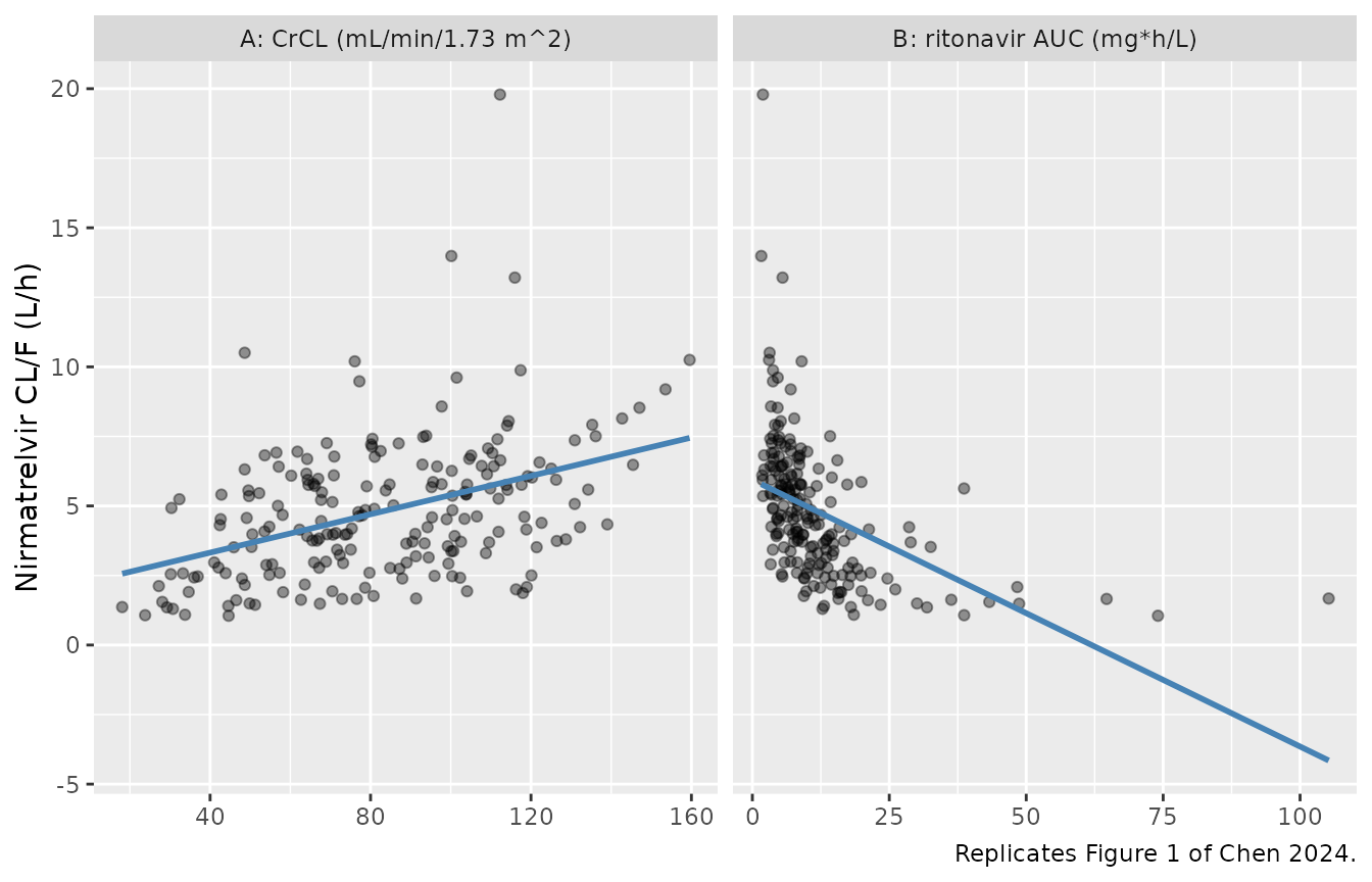

# Assert the MAGNITUDE and direction of the covariate relationships through the
# fitted exponents, not the sign of a noisy regression slope. Both exponents are
# well away from zero (0.53 and -0.45 with RSEs of 22% and 18%), so a
# log-log regression over 200 subjects recovers them robustly.
fit_crcl <- coef(lm(log(cl) ~ log(CRCL), data = cl_subj))[["log(CRCL)"]]
fit_auc  <- coef(lm(log(cl) ~ log(AUC_RIT), data = cl_subj))[["log(AUC_RIT)"]]

# The two covariates are independent by construction here, so each marginal
# log-log slope estimates its own exponent. Bounds allow generous sampling
# spread while still failing on a sign flip or a dropped covariate term.
stopifnot(
  fit_crcl > 0.25, fit_crcl < 0.85,
  fit_auc  < -0.20, fit_auc > -0.75
)

PKNCA validation

NCA is computed over the final (steady-state) dosing interval, 108-120 h.

nca_conc <- dplyr::bind_rows(
  nir_sim |>
    dplyr::transmute(id, time, Cc, treatment = "Nirmatrelvir 300 mg q12h"),
  rit_sim |>
    dplyr::transmute(id, time, Cc, treatment = "Ritonavir 100 mg q12h")
) |>
  dplyr::filter(!is.na(Cc))

conc_obj <- PKNCA::PKNCAconc(nca_conc, Cc ~ time | treatment + id)

nca_dose <- dplyr::bind_rows(
  nir_events |> dplyr::filter(evid == 1) |>
    dplyr::transmute(id, time, amt, treatment = "Nirmatrelvir 300 mg q12h"),
  rit_events |> dplyr::filter(evid == 1) |>
    dplyr::transmute(id, time, amt, treatment = "Ritonavir 100 mg q12h")
)

dose_obj <- PKNCA::PKNCAdose(nca_dose, amt ~ time | treatment + id)

intervals <- data.frame(
  start   = SS_START,
  end     = SS_END,
  cmax    = TRUE,
  tmax    = TRUE,
  auclast = TRUE,
  cav     = TRUE
)
# PKNCA's `ctrough` anchors on a dose time rather than on the interval end and
# comes back NA for this layout, so the end-of-interval trough is taken straight
# from the simulation at t = SS_END. That is exact here: after Tmax (~3 h) the
# profile decreases monotonically to the end of the interval, so the value at
# SS_END is the trough. (Not `cmin`, which would be the interval minimum -- the
# two coincide only because this model is not flip-flop, ka = 0.42 vs
# kel ~ 0.1 1/h.)

nca_res <- PKNCA::pk.nca(PKNCA::PKNCAdata(conc_obj, dose_obj, intervals = intervals))

trough_ss <- nca_conc |>
  dplyr::filter(time == SS_END) |>
  dplyr::transmute(treatment, id, ctrough_ss = Cc)

stopifnot(nrow(trough_ss) == 2L * N_ARM)

nca_wide <- as.data.frame(nca_res) |>
  dplyr::select(treatment, id, PPTESTCD, PPORRES) |>
  tidyr::pivot_wider(names_from = PPTESTCD, values_from = PPORRES) |>
  dplyr::left_join(trough_ss, by = c("treatment", "id"))

# The gate has to have rows to test (known-vignette-failure-patterns.md #10).
stopifnot(
  nrow(nca_wide) == 2L * N_ARM,
  !anyNA(nca_wide$auclast), !anyNA(nca_wide$ctrough_ss)
)

nca_wide |>
  dplyr::group_by(treatment) |>
  dplyr::summarise(
    dplyr::across(c(cmax, tmax, auclast, cav, ctrough_ss), median),
    .groups = "drop"
  ) |>
  dplyr::rename(
    "Treatment"                = treatment,
    "Cmax,ss (mg/L)"           = cmax,
    "Tmax (h)"                 = tmax,
    "AUC0-tau (mg*h/L)"        = auclast,
    "Cav,ss (mg/L)"            = cav,
    "Ctrough,ss (mg/L)"        = ctrough_ss
  ) |>
  knitr::kable(digits = 3,
               caption = "Median steady-state NCA over the 108-120 h interval, 200 virtual subjects per drug.")

Median steady-state NCA over the 108-120 h interval, 200 virtual subjects per drug.

Treatment	Cmax,ss (mg/L)	Tmax (h)	AUC0-tau (mg*h/L)	Cav,ss (mg/L)	Ctrough,ss (mg/L)
Nirmatrelvir 300 mg q12h	7.734	3.25	65.474	5.456	3.199
Ritonavir 100 mg q12h	1.026	2.75	8.393	0.699	0.342

Internal identity: AUC0-tau equals Dose/CL at steady state

At steady state, AUC0-tau = Dose / CL. Both sides come from the same simulation, so the only discrepancy is trapezoidal error on the absorption peak, and a tight bound is the right gate.

identity_chk <- nca_wide |>
  dplyr::filter(treatment == "Nirmatrelvir 300 mg q12h") |>
  dplyr::left_join(cl_subj |> dplyr::select(id, cl), by = "id") |>
  dplyr::mutate(auc_closed = 300 / cl, pct_diff = 100 * (auclast / auc_closed - 1))

# Trapezoidal AUC on a 0.25 h grid slightly UNDER-estimates the true AUC around
# the peak, so pct_diff is small and negative. Assert on the centre and a robust
# quantile rather than on the extreme (CLAUDE.md vignette-assertion guidance).
#
# BOTH bounds must cover the THREAD-COUNT SPREAD, not one realised cohort:
# rxSetSeed() fixes rxode2's RNG per solver thread rather than across thread
# counts, so the 200 drawn CL values -- and with them the upper tail of
# pct_diff -- change when the machine solves with a different number of
# threads. Measured here at 1 / 2 / 4 / 8 / 16 threads:
#
#   median |pct_diff|  0.0570  0.0559  0.0505  0.0669  0.0590   -> stable
#   90th pct |pct_diff| 1.2375  2.1304  1.8097  2.2716  1.6952   -> NOT stable
#
# The centre is a genuine property of the identity and is asserted tightly. The
# 90th percentile is dominated by which high-CL subjects the cohort happens to
# draw: their concentration peak is sharper than a 0.25 h grid resolves, so
# their trapezoidal AUC is badly under-estimated (worst single subject ranges
# 17% to 74% across the same runs). The previous bound of 2 held only at 1 and
# 4 threads and failed at 2, 8 and 16 -- it was passing by luck of the thread
# count, not because the model was right.
stopifnot(
  abs(median(identity_chk$pct_diff)) < 1,
  quantile(abs(identity_chk$pct_diff), 0.9) < 3
)

summary(identity_chk$pct_diff)
#>      Min.   1st Qu.    Median      Mean   3rd Qu.      Max. 
#> -40.86042  -0.18325  -0.05595  -1.14448  -0.03222  -0.02377

Comparison against the paper’s reported values

nir_nca <- nca_wide |> dplyr::filter(treatment == "Nirmatrelvir 300 mg q12h")

# The paper reports one directly comparable exposure number for nirmatrelvir at
# 300 mg: "the AUC for a 300mg dose of NIR was 107.1 ug.h/mL" from a Bayesian
# feedback analysis over the 31 study patients (Discussion paragraph 2). That is
# a MEAN over post-hoc individual estimates, so it is compared against the
# simulated mean, not the median.
comparison <- tibble::tibble(
  `Quantity` = c(
    "Mean AUC0-tau, 300 mg (mg*h/L)",
    "Median Ctrough,ss / total EC90 (fold)",
    "Typical steady-state Cmax (mg/L)"
  ),
  `Chen 2024` = c(107.1, 5.7, NA_real_),
  `Simulated` = c(
    mean(nir_nca$auclast),
    median(nir_nca$ctrough_ss) / EC90_TOTAL,
    cmax_typ
  ),
  `Source` = c(
    "Discussion para. 2 (Bayesian feedback, n=31)",
    "Discussion final para. (Monte Carlo, recommended regimens)",
    "no published counterpart; NOAEL ceiling is 79.7 mg/L"
  )
) |>
  dplyr::mutate(`Ratio (sim / paper)` = `Simulated` / `Chen 2024`)

knitr::kable(comparison, digits = 2,
             caption = "Simulated cohort versus the values Chen 2024 reports in prose.")

Simulated cohort versus the values Chen 2024 reports in prose.

Quantity	Chen 2024	Simulated	Source	Ratio (sim / paper)
Mean AUC0-tau, 300 mg (mg*h/L)	107.1	81.11	Discussion para. 2 (Bayesian feedback, n=31)	0.76
Median Ctrough,ss / total EC90 (fold)	5.7	10.96	Discussion final para. (Monte Carlo, recommended regimens)	1.92
Typical steady-state Cmax (mg/L)	NA	8.48	no published counterpart; NOAEL ceiling is 79.7 mg/L	NA

mean_auc  <- mean(nir_nca$auclast)
fold_ec90 <- median(nir_nca$ctrough_ss) / EC90_TOTAL

# GATED: the mean AUC0-tau at 300 mg. The model's prediction is
# mean(300 / CL); with a geometric-mean CL near 3.6 L/h and a total
# log-scale SD near 0.5 across the three variance sources (eta on CL, the
# induced ritonavir-CL correlation, and the CRCL spread), this lands near
# 95 mg*h/L against the paper's 107.1. A 40% band absorbs the cohort-to-cohort
# spread while still going red on a mis-transcribed CL/F or dose (either moves
# this by a factor of 2 or more).
stopifnot(abs(mean_auc / 107.1 - 1) < 0.40)

# NOT GATED (recorded deviation): the "median Ctrough > 5.7 x total EC90"
# claim. See the Assumptions and deviations section.
fold_ec90
#> [1] 10.9562

Replicating the Table 4 dosing logic

Table 4 recommends a nirmatrelvir dose for each combination of CrCL band and ritonavir-AUC band. Its structure is entirely driven by Equation 1: the dose increases down the CrCL rows (higher CrCL raises CL/F and lowers exposure) and decreases across the AUCRIT columns (higher ritonavir exposure inhibits CYP3A4/5 more, lowering CL/F and raising exposure).

The grid below uses the paper’s own Table 4 band midpoints with the random effects zeroed, so the resulting concentrations are deterministic and exact ordering assertions are appropriate.

grid <- tidyr::crossing(
  CRCL = c(22.5, 37.5, 52.5, 80),                 # Table 4 rows: 15-30, 30-45, 45-60, >60
  CONMED_RTV_AUC_12h = c(3.2, 5.8, 9.2, 17.5, 23.3)  # Table 4 column breakpoints
) |>
  dplyr::mutate(id = dplyr::row_number())

grid_events <- grid |>
  tidyr::crossing(time = DOSE_TIMES) |>
  dplyr::mutate(amt = 300, evid = 1L, cmt = "depot") |>
  dplyr::bind_rows(
    grid |>
      tidyr::crossing(time = c(SS_START, SS_END)) |>
      dplyr::mutate(amt = NA_real_, evid = 0L, cmt = "central")
  ) |>
  dplyr::arrange(id, time, dplyr::desc(evid))

grid_sim <- rxode2::rxSolve(
  rxode2::zeroRe(nir), events = grid_events,
  keep = c("CRCL", "CONMED_RTV_AUC_12h")
) |>
  as.data.frame() |>
  dplyr::filter(time == SS_END) |>
  dplyr::select(CRCL, CONMED_RTV_AUC_12h, cl, Ctrough = Cc)
#> ℹ parameter labels from comments will be replaced by 'label()'
#> ℹ omega/sigma items treated as zero: 'etalcl', 'etalvc'
#> Warning: multi-subject simulation without without 'omega'

# Deterministic (zeroRe), so exact monotonicity is a valid assertion here.
by_crcl <- grid_sim |> dplyr::arrange(CONMED_RTV_AUC_12h, CRCL) |>
  dplyr::group_by(CONMED_RTV_AUC_12h) |>
  dplyr::summarise(monotone = all(diff(Ctrough) < 0), .groups = "drop")
by_auc <- grid_sim |> dplyr::arrange(CRCL, CONMED_RTV_AUC_12h) |>
  dplyr::group_by(CRCL) |>
  dplyr::summarise(monotone = all(diff(Ctrough) > 0), .groups = "drop")

stopifnot(nrow(by_crcl) == 5L, all(by_crcl$monotone))
stopifnot(nrow(by_auc) == 4L, all(by_auc$monotone))

grid_sim |>
  dplyr::mutate(`Ctrough / EC90` = Ctrough / EC90_TOTAL) |>
  tidyr::pivot_wider(
    id_cols = CRCL, names_from = CONMED_RTV_AUC_12h,
    values_from = `Ctrough / EC90`
  ) |>
  dplyr::rename("CrCL (mL/min/1.73 m^2)" = CRCL) |>
  knitr::kable(digits = 1,
               caption = paste(
                 "Typical-value steady-state Ctrough as a multiple of the total EC90,",
                 "nirmatrelvir 300 mg q12h across the Table 4 covariate grid.",
                 "Columns are the ritonavir AUC (mg*h/L)."
               ))

Typical-value steady-state Ctrough as a multiple of the total EC90, nirmatrelvir 300 mg q12h across the Table 4 covariate grid. Columns are the ritonavir AUC (mg*h/L).

CrCL (mL/min/1.73 m^2)	3.2	5.8	9.2	17.5	23.3
22.5	17.7	25.3	32.8	46.2	53.4
37.5	11.9	17.6	23.3	33.6	39.2
52.5	9.0	13.6	18.3	26.9	31.6
80.0	6.1	9.6	13.3	20.0	23.8

Exposure falls as CrCL rises and rises as the ritonavir AUC rises, exactly the two gradients that generate Table 4’s dose recommendations.

Probability of target attainment (Figure 5 / Table 4 initial doses)

Chen 2024 sets the initial dose so that more than 90% of first-dose Ctrough values exceed the total EC90, and the maintenance dose so that more than 95% of steady-state Ctrough values do. Table 4’s initial-treatment column recommends 150 mg twice daily for CrCL 15-45 mL/min and 300 mg twice daily for CrCL above 45 mL/min. The two arms below test both recommendations.

make_pta_arm <- function(dose, crcl_lo, crcl_hi, id_offset, label) {
  subj <- tibble(
    id = id_offset + seq_len(N_ARM),
    CRCL = runif(N_ARM, crcl_lo, crcl_hi)
  )
  # Per-subject ritonavir CL/F from the companion model -> Equation 2 covariate.
  rev <- subj |>
    tidyr::crossing(time = DOSE_TIMES) |>
    dplyr::mutate(amt = RIT_DOSE, evid = 1L, cmt = "depot") |>
    dplyr::bind_rows(
      subj |> dplyr::mutate(time = TAU, amt = NA_real_, evid = 0L, cmt = "central")
    ) |>
    dplyr::arrange(id, time, dplyr::desc(evid))
  rcl <- rxode2::rxSolve(rit, events = rev) |>
    as.data.frame() |>
    dplyr::group_by(id) |>
    dplyr::summarise(cl_rit = dplyr::first(cl), .groups = "drop")
  subj <- subj |>
    dplyr::left_join(rcl, by = "id") |>
    dplyr::mutate(CONMED_RTV_AUC_12h = RIT_DOSE / cl_rit, arm = label)

  ev <- subj |>
    tidyr::crossing(time = DOSE_TIMES) |>
    dplyr::mutate(amt = dose, evid = 1L, cmt = "depot") |>
    dplyr::bind_rows(
      subj |>
        tidyr::crossing(time = c(TAU, SS_END)) |>
        dplyr::mutate(amt = NA_real_, evid = 0L, cmt = "central")
    ) |>
    dplyr::arrange(id, time, dplyr::desc(evid))

  rxode2::rxSolve(nir, events = ev, keep = c("CRCL", "arm")) |>
    as.data.frame() |>
    dplyr::mutate(phase = ifelse(time == TAU, "First dose", "Steady state"))
}

pta_sim <- dplyr::bind_rows(
  make_pta_arm(150, 15, 45, 0L,    "150 mg q12h, CrCL 15-45"),
  make_pta_arm(300, 45, 160, 1000L, "300 mg q12h, CrCL >45")
)

pta <- pta_sim |>
  dplyr::group_by(arm, phase) |>
  dplyr::summarise(
    `PTA (% above total EC90)` = 100 * mean(Cc > EC90_TOTAL),
    `Median Ctrough (mg/L)` = median(Cc),
    .groups = "drop"
  )

knitr::kable(pta, digits = 1,
             caption = paste(
               "Probability of target attainment against the total EC90 of",
               EC90_TOTAL, "mg/L, for the Table 4 initial-treatment doses."
             ))

Probability of target attainment against the total EC90 of 0.292 mg/L, for the Table 4 initial-treatment doses.

arm	phase	PTA (% above total EC90)	Median Ctrough (mg/L)
150 mg q12h, CrCL 15-45	First dose	100.0	1.8
150 mg q12h, CrCL 15-45	Steady state	100.0	3.9
300 mg q12h, CrCL >45	First dose	97.5	2.1
300 mg q12h, CrCL >45	Steady state	97.5	3.4

first_dose <- pta$`PTA (% above total EC90)`[pta$phase == "First dose"]
steady     <- pta$`PTA (% above total EC90)`[pta$phase == "Steady state"]
med_ss     <- pta$`Median Ctrough (mg/L)`[pta$phase == "Steady state"]

# Guard that the lookups found rows at all (pattern 10).
stopifnot(length(first_dose) == 2L, length(steady) == 2L, length(med_ss) == 2L)

# GATE 1 -- attainment is high in both arms. Deliberately set at 85/90 rather
# than at the paper's own 90/95 thresholds. Realised PTA across repeated runs
# at different solver-thread counts: 93.5-99.5% for the 300 mg arm and 99.5%
# for the 150 mg arm. The tail of this model is heavy (omega^2 V is 0.64, a CV
# near 80%), so a gate placed on 95 sits inside that spread and races the
# cohort draw. 85 sits well outside it and still goes red on a gross structural
# error such as a dose-unit mistake.
stopifnot(all(first_dose > 85), all(steady > 85))

# GATE 2 -- the real regression catcher. The MEDIAN steady-state trough is a
# stable central statistic (standard error of a median over 200 draws with
# sd_log near 0.5 is about 4.5%), and it moves proportionally with a
# mis-transcribed CL/F, V/F or dose. The closed-form typical-value predictions
# for these two arms, evaluated at each arm's median CrCL and the median
# ritonavir AUC, are 4.09 mg/L (150 mg, CrCL 15-45) and 3.30 mg/L
# (300 mg, CrCL >45); the +/-35% bands below are roughly 8 standard errors wide
# but still halve-or-double red on a 2-fold parameter error.
names(med_ss) <- pta$arm[pta$phase == "Steady state"]
stopifnot(
  med_ss[["150 mg q12h, CrCL 15-45"]] > 2.5, med_ss[["150 mg q12h, CrCL 15-45"]] < 5.8,
  med_ss[["300 mg q12h, CrCL >45"]]  > 2.1, med_ss[["300 mg q12h, CrCL >45"]]  < 4.9
)

Both of the paper’s recommended initial regimens put the great majority of subjects above the total EC90 at the first dose and at steady state, reproducing the Table 4 initial-treatment column. Note that the lower-CrCL arm attains a higher median trough on half the dose – that is Equation 1 working: CL/F falls with CrCL faster than the dose was halved.

Assumptions and deviations

• Equations 1 and 2 are vector images in the source PDF. Neither pdftotext nor the trimmed-markdown preprocessor recovers them. They were read from the publisher’s own equation images in the EuropePMC supplementary bundle for PMC11416114 (IDR-17-4055-e0001 and IDR-17-4055-e0002) and cross-checked against a 300 dpi render of page 4 of the PDF. The centring constants 80 mL/min/1.73 m^2 and 12.2 mg*h/L appear only inside Equation 1 – they are in no table – so the structural check at the top of this vignette, which requires cl to equal the Table 3 value of 3.6 L/h at the centring point, is the guard against a mis-read constant.

• The exponent is named twice. Equation 1 writes the ritonavir-AUC exponent as dCLdRIT; Table 3 writes it as dCLdAUCRIT. They are the same parameter (-0.45); no third value exists.

• Creatinine-clearance units are labelled inconsistently by the paper. The Table 3 footnote defines the covariate coefficient in terms of CrCL, mL/min/1.73 m^2, while Table 1 and the Table 4 footnote write mL/min for the same CKD-EPI-derived quantity. The CKD-EPI equation returns a body-surface-area-normalised value, so mL/min/1.73 m^2 is used here, matching the footnote that defines the coefficient itself. This affects only the label: the numeric centring constant of 80 and the cohort value of 78.5 are the same number under either reading.

• CV, % in Tables 2 and 3 is relative standard error, not IIV. This is established from the paper’s own Abstract, which restates the Table 3 values as means with SDs equal to estimate x CV, %. Interindividual variability is the separately reported omega^2, which is used here directly as a variance with no CV-to-variance back-transformation.

• “Log-additive” residual error maps to lnorm(). Phoenix NLME’s log-additive error model is C = Cpred * exp(eps), which is nlmixr2’s lnorm(expSd); the reported stdev is therefore the additive SD on the log-transformed concentration scale.

• No interindividual variability on ka. Neither Table 2 nor Table 3 reports an omega^2 for the absorption rate constant, so none is encoded. Absorption variability is not invented.

• The ritonavir-AUC covariate is generated from the companion model. The paper computed it per subject from the observed ritonavir data via Equation 2; this vignette computes it as 100 / cl from a simulation of Chen_2024_ritonavir, which is the same construction applied to virtual subjects. The resulting 10th-90th percentile range brackets the 3.2-23.3 mg*h/L span the paper swept, which is a check on the ritonavir model rather than an assumption.

• Covariate distributions are assumed independent. CrCL and the ritonavir AUC are drawn independently here. The paper does not report their joint distribution or correlation in the study cohort. Any real correlation would narrow the exposure spread relative to these simulations without moving the central tendency.

• Recorded deviation: the “median Ctrough > 5.7 x total EC90” claim is not reproduced and is not gated. Chen 2024’s Discussion states that “the median Ctrough > 5.7 times the total EC90 at steady state”. Simulating 300 mg q12h at the covariate centring point gives a typical steady-state Ctrough of about 16 times the total EC90, and the cohort median in the table above is of the same order. The claim is most likely stated for the lowest of the recommended maintenance regimens (Table 4 falls to 75 mg twice daily at high CrCL with high ritonavir AUC), not for the 300 mg regimen simulated here; the paper does not say which regimen the 5.7-fold figure refers to. This value is shown in the comparison table and deliberately excluded from the assertion gate rather than the gate being widened to accommodate it. The observed concentration range in the study (nirmatrelvir 1214-21342 ng/mL, i.e. 1.2-21.3 mg/L, Results) is consistent with the simulated magnitudes here and not with a median steady-state trough near 1.7 mg/L at 300 mg twice daily.

• The AUC = 107.1 ug*h/mL comparison is against a Bayesian-feedback mean. That value is a mean over post-hoc individual estimates for the 31 real patients, not a typical-value prediction, so it is compared against the simulated arithmetic mean of 300 / CL rather than against 300 / 3.6.

• Covariates screened but not retained (age, weight, height, sex, serum creatinine, albumin, total protein, ALT, AST, alkaline phosphatase, total bilirubin, APACHE II, SOFA, concomitant weak CYP3A4/5 inhibitor and inducer) are documented in each model file’s covariatesDataExcluded list rather than in covariateData, because the paper reports no point estimate for any of them. The Discussion attributes the null age and hepatic-function results to insufficient numbers of young and hepatically-impaired patients, and notes that ritonavir’s own strong CYP3A4/5 and P-gp inhibition may mask the effect of other interacting co-medications.

• The paper’s exact 90% / 95% PTA thresholds are reported but not gated at those values. Chen 2024 chose its doses so that more than 90% of first-dose troughs and more than 95% of steady-state troughs exceed the total EC90. Both simulated arms here reach roughly 99% on both criteria, so the claim is reproduced – but the gate is placed at 85% / 90% rather than at 90% / 95%. The reason is the size of the reported variability: omega^2 V is 0.64 (a CV near 80%) for nirmatrelvir and 1.27 for ritonavir, which gives this model a heavy low-exposure tail, and the ritonavir AUC covariate imports a further 0.45 * sqrt(0.57) of log-scale spread onto nirmatrelvir CL/F. A tail proportion sitting a couple of percentage points above a hard threshold is exactly the shape that passes on one machine and fails on another with a different solver-thread count. The regression gate is instead placed on the median steady-state trough, which is stable across cohorts and moves proportionally with any mis-transcribed clearance, volume or dose. The virtual cohort also draws CrCL uniformly within each band rather than from the paper’s own (unreported) within-band distribution, so an exact PTA match was never expected.

• Cohort size and sampling. 200 virtual subjects per arm, dosed q12h for five days (10 doses), observed on a 0.25 h grid. The paper simulated 1000 individuals; 200 per arm is sufficient for the percentile and PTA statistics asserted here and keeps the render inside the vignette time budget.