Benznidazole in neonates, infants and children (Altcheh 2023)
Source:vignettes/articles/Altcheh_2023_benznidazole.Rmd
Altcheh_2023_benznidazole.RmdModel and source
- Citation: Altcheh J, Moscatelli G, Caruso M, Moroni S, Bisio M, Miranda MR, Monla C, Vaina M, Valdez M, Moran L, Ramirez T, Ledesma Patino O, Riarte A, Gonzalez N, Fernandes J, Alves F, Ribeiro I, Garcia-Bournissen F. Population pharmacokinetics of benznidazole in neonates, infants and children using a new pediatric formulation. PLoS Neglected Tropical Diseases. 2023;17(5):e0010850. doi:10.1371/journal.pntd.0010850.
- Description: One-compartment population PK model with first-order absorption and first-order elimination for oral benznidazole in neonates, infants and children (0-12 years) with Chagas disease treated with a new 12.5 mg dispersible pediatric formulation (Altcheh 2023; PEDCHAGAS network, NCT01549236, n = 81). Apparent clearance CL/F = 2.1 L/h at the 70 kg allometric reference, scaled by (WT/70)^0.75 with the exponent fixed at the theory-based 3/4. Apparent volume of distribution V/F is a LINEAR function of body weight, V/F = 1.75 + 0.804 * WT (L), not a power function. Absorption rate constant Ka = 1.22 1/h. Inter-individual variability is on Ka (61.9% CV), V/F (47.4% CV) and CL/F (38.3% CV); residual error is proportional (37.1% CV). Weight was the only covariate retained; age, sex, postmenstrual age, dose, tablet formulation and study center were screened and not retained.
- Article: https://doi.org/10.1371/journal.pntd.0010850
- Trial registry: ClinicalTrials.gov NCT01549236 (PEDCHAGAS network, Argentina).
mod <- readModelDb("Altcheh_2023_benznidazole")()
mod
#>  ── rxode2-based free-form 2-cmt ODE model ──────────────────────────────────────
#>  ── Initalization: ──
#> Fixed Effects ($theta):
#>       lka       lcl       lvc   e_wt_vc   e_wt_cl    propSd
#> 0.1988509 0.7419373 0.5596158 0.8040000 0.7500000 0.3710000
#>
#> Omega ($omega):
#>          etalka   etalvc   etalcl
#> etalka 0.324371 0.000000 0.000000
#> etalvc 0.000000 0.202676 0.000000
#> etalcl 0.000000 0.000000 0.136879
#>
#> States ($state or $stateDf):
#>   Compartment Number Compartment Name
#> 1                  1            depot
#> 2                  2          central
#>  ── μ-referencing ($muRefTable): ──
#>   theta    eta level
#> 1   lka etalka    id
#> 2   lcl etalcl    id
#>
#>  ── Model (Normalized Syntax): ──
#> function() {
#>     compartmentData <- list(depot = list(analyte = "benznidazole",
#>         units = "mg", specimen = "administration site", verified = TRUE),
#>         central = list(analyte = "benznidazole", units = "mg",
#>             specimen = "whole blood", verified = TRUE))
#>     covariateData <- list(WT = list(description = "Total body weight",
#>         units = "kg", type = "continuous", reference_category = NULL,
#>         notes = "The only covariate retained in the final model (Altcheh 2023 Results, 'Covariate modeling'). Enters CL/F allometrically as (WT/70)^0.75 with the exponent FIXED at the theory-based 3/4 value, and enters V/F LINEARLY as 1.75 + 0.804 * WT -- note the V/F relationship is additive on the natural scale, NOT a power function, so V/F is not proportional to weight. Time-varying: because weight was recorded only at the start of the 60-day dosing period, intermediate weights for children under 18 months were interpolated from the WHO weight-for-age percentile curves following each child's own percentile (Altcheh 2023 Methods, 'Covariate model').",
#>         source_name = "Wt"))
#>     covariatesDataExcluded <- list(AGE = list(description = "Subject age",
#>         units = "years", type = "continuous", reference_category = NULL,
#>         notes = "Screened on V/F and CL/F. Altcheh 2023 Results: 'Addition of age as a covariate for V/F did not improve the fit beyond the effect of weight.' CL/F correlates strongly with age (Fig 4) but only because age and weight are collinear in children; weight is the retained covariate. Register canonical carries years; the paper tabulates age in months (Table 1).",
#>         source_name = "Age"), SEXF = list(description = "Sex indicator (1 = female, 0 = male)",
#>         units = "(binary)", type = "binary", reference_category = "0 (male)",
#>         notes = "Screened as 'gender' and not retained. Neither Cmax nor trough concentrations differed between girls and boys (Mann-Whitney p > 0.05; Altcheh 2023 Results). Cohort was 47/81 (58.0%) female (Table 1).",
#>         source_name = "gender"), PAGE = list(description = "Postmenstrual age",
#>         units = "months", type = "continuous", reference_category = NULL,
#>         notes = "Screened on CL/F via an empirical sigmoidal PMA-CL/F relationship and not retained; the allometric weight model fit marginally better and was chosen for parsimony (Altcheh 2023 Results, 'Covariate modeling'). Altcheh 2023 estimated PMA by adding 9 months to the actual postnatal age in months at each blood sampling timepoint (Methods, 'Covariate model'), so this column is time-varying and carried in MONTHS, matching the register default.",
#>         source_name = "PMA"))
#>     description <- "One-compartment population PK model with first-order absorption and first-order elimination for oral benznidazole in neonates, infants and children (0-12 years) with Chagas disease treated with a new 12.5 mg dispersible pediatric formulation (Altcheh 2023; PEDCHAGAS network, NCT01549236, n = 81). Apparent clearance CL/F = 2.1 L/h at the 70 kg allometric reference, scaled by (WT/70)^0.75 with the exponent fixed at the theory-based 3/4. Apparent volume of distribution V/F is a LINEAR function of body weight, V/F = 1.75 + 0.804 * WT (L), not a power function. Absorption rate constant Ka = 1.22 1/h. Inter-individual variability is on Ka (61.9% CV), V/F (47.4% CV) and CL/F (38.3% CV); residual error is proportional (37.1% CV). Weight was the only covariate retained; age, sex, postmenstrual age, dose, tablet formulation and study center were screened and not retained."
#>     population <- list(species = "human", n_subjects = 81L, n_studies = 1L,
#>         n_observations = 383L, age_range = "0-12 years (14 newborns < 1 month of age; 41/81 under 2 years)",
#>         age_median = "16 months (IQR 2.76-75.6); mean 42.3 months (SD 47.3)",
#>         weight_range = "not reported as a range; median 12 kg (IQR 8.1-23)",
#>         weight_mean = "16.69 kg (SD 12.8)", sex_female_pct = 58,
#>         disease_state = "Children 0-12 years with Chagas disease (Trypanosoma cruzi infection), treatment-naive, all asymptomatic without cardiac symptoms or other organ involvement. Diagnosis by at least two positive serologic tests (age > 8 months) or by direct microhematocrit parasite detection (age < 8 months). 69/80 (85%) were qPCR-positive for T. cruzi DNA at enrolment. Excluded: pregnancy, investigational drug within the prior month, cardiovascular / hepatic / neurologic / endocrine or other major systemic disease, immunocompromise.",
#>         dose_range = "Oral benznidazole 7.5 mg/kg/day divided into two daily doses for 60 days (actual administered dose mean 7.35 mg/kg, SD 0.65; Table 1). Formulation assigned by a 14 kg enrolment weight cut-off: 12.5 mg dispersible pediatric tablet below, 100 mg non-dispersible tablet at or above (LAFEPE, Brazil).",
#>         sampling = "Sparse design, 5 blood samples per child at random times within pre-specified windows: Day 0 at 2-5 h after the first dose; Day 7 and Day 30 at steady state, each between pre-dose and 8 h post-dose; and two samples 12-24 h AFTER THE FINAL dose on Day 60 (i.e. during washout, not steady-state troughs). 387 samples collected, 383 quantifiable; the 4 BLQ samples (1%) were excluded from the PK analysis after confirming they did not change the fit. Whole dried blood spots on Whatman 903 paper, LC-ESI-MS/MS, linear 50-20,000 ng/mL, LLOQ 50 ng/mL.",
#>         regions = "Five pediatric centers in Argentina (PEDCHAGAS Network), all in areas with certified vector control to avoid confounding by re-infection. Enrolment May 2011 - August 2012.",
#>         notes = "Open-label single-group interventional trial, ClinicalTrials.gov NCT01549236. Baseline demographics from Altcheh 2023 Table 1; final parameter estimates from Table 2 and the three displayed equations that immediately precede it. Covariates screened and NOT retained: age, sex, postmenstrual age, dose per kg, total daily benznidazole dose, study center, and tablet formulation (12.5 mg dispersible vs 100 mg). Table 1 and the Results text disagree on two demographic counts (median age 16 vs 22 months; 44 vs 46 patients on the 12.5 mg formulation); Table 1 is used here because its formulation split, 44/81, is the one consistent with the 54% the text itself reports. Neither value is used by model().")
#>     reference <- "Altcheh J, Moscatelli G, Caruso M, Moroni S, Bisio M, Miranda MR, Monla C, Vaina M, Valdez M, Moran L, Ramirez T, Ledesma Patino O, Riarte A, Gonzalez N, Fernandes J, Alves F, Ribeiro I, Garcia-Bournissen F. Population pharmacokinetics of benznidazole in neonates, infants and children using a new pediatric formulation. PLoS Neglected Tropical Diseases. 2023;17(5):e0010850. doi:10.1371/journal.pntd.0010850."
#>     units <- list(time = "h", dosing = "mg", concentration = "mg/L")
#>     vignette <- "Altcheh_2023_benznidazole"
#>     ini({
#>         lka <- 0.198850858745165
#>         label("Absorption rate constant Ka (1/h)")
#>         lcl <- 0.741937344729377
#>         label("Apparent oral clearance CL/F (L/h) at the 70 kg allometric reference")
#>         lvc <- 0.559615787935423
#>         label("Intercept b0 of the linear V/F-weight relationship (L, apparent volume at extrapolated WT = 0)")
#>         e_wt_vc <- 0.804
#>         label("Linear additive effect of WT on V/F (L per kg body weight)")
#>         e_wt_cl <- fix(0.75)
#>         label("Allometric exponent of WT on CL/F (unitless, the theory-based 3/4)")
#>         propSd <- c(0, 0.371)
#>         label("Proportional residual error on Cc (fraction CV)")
#>         etalka ~ 0.324371
#>         etalvc ~ 0.202676
#>         etalcl ~ 0.136879
#>     })
#>     model({
#>         ka <- exp(lka + etalka)
#>         cl <- exp(lcl + etalcl) * (WT/70)^e_wt_cl
#>         vc <- (exp(lvc) + e_wt_vc * WT) * exp(etalvc)
#>         kel <- cl/vc
#>         d/dt(depot) <- -ka * depot
#>         d/dt(central) <- ka * depot - kel * central
#>         Cc <- central/vc
#>         Cc ~ prop(propSd)
#>     })
#> }
Population
Altcheh 2023 enrolled 81 children aged 0-12 years with Chagas disease at five pediatric centers in Argentina between May 2011 and August 2012. Enrolment was stratified by age so that roughly half the cohort was under 2 years old: 41/81 (51%) were under 2 years, including 14 newborns under 1 month. Median age was 16 months (IQR 2.76-75.6) and median weight 12 kg (IQR 8.1-23; mean 16.69, SD 12.8). 47/81 (58.0%) were female. All patients were asymptomatic and treatment-naive; 69/80 (85%) were qPCR-positive for T. cruzi DNA at enrolment.
Every patient received oral benznidazole 7.5 mg/kg/day divided into two daily doses for 60 days. A 14 kg enrolment-weight cut-off decided the formulation: the new 12.5 mg dispersible pediatric tablet below it (44/81, 54%) and the 100 mg non-dispersible adult tablet at or above it (37/81, 46%).
Five blood samples per child were drawn at random times inside pre-specified windows: one 2-5 h after the first dose on Day 0; one each on Day 7 and Day 30 at steady state, between pre-dose and 8 h post-dose; and two 12-24 h after the final dose on Day 60. That last window matters for interpretation: the paper’s “Cmin (trough)” is measured during washout after treatment stopped, not as a steady-state pre-dose trough. Benznidazole was quantified in whole dried blood spots (Whatman 903 paper) by LC-ESI-MS/MS, LLOQ 50 ng/mL. Of 387 samples, 383 were quantifiable; the 4 BLQ samples (1%) were excluded from the PK analysis.
The same information is available programmatically via the model’s
population metadata
(readModelDb("Altcheh_2023_benznidazole")()$population).
Source trace
The per-parameter origin is recorded inline next to each
ini() entry in
inst/modeldb/specificDrugs/Altcheh_2023_benznidazole.R. The
table below collects them in one place for review. Altcheh 2023 prints
the final model as three displayed equations sitting between Fig 3 and
Table 2, with the same point estimates repeated in Table 2.
| Equation / parameter | Value | Source location |
|---|---|---|
lka (= log(1.22)) |
Ka = 1.22 1/h | Altcheh 2023 displayed equation Ka (/h) = 1.22; Table 2
row “Ka (h-1)”, 1.22 [95% CI 0.91; 1.65]. |
lcl (= log(2.1)) |
CL/F = 2.1 L/h at WT = 70 kg | Altcheh 2023 displayed equation
CL/F (L/h) = 2.1 (L/h) x (Wt (Kg) / 70 (Kg))^0.75; Table 2
row “CL/F (L/hr)”, 2.1 [1.89; 2.39]. Results text confirms “The
estimated BNZ clearance for a 70 Kg adult was 2.1 L/h”. |
lvc (= log(1.75)) |
V/F intercept b0 = 1.75 L | Altcheh 2023 displayed equation
V/F (L) = 1.75 (L) + 0.804 (L/Kg) x Wt (Kg); Table 2 row
“V/F (L)”, b0 = 1.75 [0; 4.48]. |
e_wt_vc |
V/F slope b1 = 0.804 L/kg | Same displayed V/F equation; Table 2 b1 = 0.804 [0.62; 0.99]. Linear additive on the natural scale, not a power function. |
e_wt_cl |
0.75, FIXED | Altcheh 2023 Methods “Covariate model”: “An allometric scaling approach of weight on apparent oral clearance (CL/F) (by using the theory-based allometric exponent of 3/4) was used”. Printed as a literal exponent in the displayed CL/F equation; Table 2 gives no CI for it. |
etalka variance |
log(1 + 0.619^2) = 0.324371 | Table 2 IIV column, Ka = 61.9% CV. Methods: “Inter-individual variability in PK parameters was described using exponential error models”. |
etalvc variance |
log(1 + 0.474^2) = 0.202676 | Table 2 IIV column, V/F = 47.4% CV. |
etalcl variance |
log(1 + 0.383^2) = 0.136879 | Table 2 IIV column, CL/F = 38.3% CV. |
propSd |
0.371 (fraction CV) | Table 2 row “Residual error (Proportional)”, 37.1% [34.6; 41.7%]. Methods: “The residual variability was described using a proportional error model”. |
d/dt(depot), d/dt(central)
|
one compartment, first-order absorption and elimination | Altcheh 2023 Results, “BNZ PK modeling and simulation”: two- and three-compartment models “failed to decrease the Objective Function”, so “A one compartment model with first order oral absorption was therefore adopted”. |
| Reference weight 70 kg | hardcoded in (WT / 70)^e_wt_cl
|
Printed literally as 70 (Kg) in the displayed CL/F
equation. |
Note the encoding of V/F. Because Altcheh 2023 models volume as an
additive function of weight, lvc carries the
intercept b0 (the extrapolated volume at
WT = 0), not a typical volume at some reference weight, and
e_wt_vc carries the slope in L per kg.
Inside model() the bracket is formed on the natural scale
before the exponential IIV multiplier is applied:
This is the additive-covariate encoding established by
Goggin_2004_emfilermin.R. A consequence worth stating
explicitly is that V/F is not proportional to body
weight: weight-normalised V/F falls from 1.24 L/kg at 4 kg to 0.83 L/kg
at 30 kg.
Virtual cohort
The cohort reproduces Altcheh 2023’s stratified enrolment design: 41/81 of subjects under 2 years old, with each stratum’s age distribution matched to the corresponding sub-row of Table 1 (under 2 years: median 2.76 months, IQR 0.84-4.68; over 2 years: median 79.8 months, IQR 51-114).
Weights are not reported per subject, so they are generated from the WHO Child Growth Standards / 2007 Growth Reference weight-for-age medians (sexes averaged, interpolated over age) with log-normal scatter representing percentile spread. This is external reference data, not paper data – it is used only to construct a plausible covariate distribution, and the construction is checked below against the demographic totals Altcheh 2023 does report.
# WHO weight-for-age median (kg) by age (months), sexes averaged. External
# reference data (WHO Child Growth Standards 0-5 y; WHO Growth Reference
# 5-19 y), NOT from Altcheh 2023 -- used only to build the virtual cohort.
who_age_mo <- c(0, 1, 2, 3, 6, 9, 12, 18, 24, 36, 48, 60, 72, 84, 96, 108, 120, 132, 144)
who_wt_kg  <- c(3.3, 4.4, 5.5, 6.3, 7.8, 8.8, 9.5, 10.8, 12.0, 14.2, 16.2,
                18.3, 20.5, 22.9, 25.6, 28.6, 32.0, 35.9, 40.1)
whoMedianWt <- function(age_mo) {
  stats::approx(who_age_mo, who_wt_kg, xout = age_mo, rule = 2)$y
}

set.seed(20230531)
n       <- 200L
n_young <- round(n * 41 / 81)   # Altcheh 2023 Table 1: 41/81 under 2 years
n_old   <- n - n_young

# Under-2 stratum: log-normal matched to median 2.76 mo, IQR 0.84-4.68 mo.
sd_young  <- (log(4.68) - log(0.84)) / (2 * stats::qnorm(0.75))
age_young <- pmin(pmax(exp(stats::rnorm(n_young, log(2.76), sd_young)), 0.03), 23.9)

# Over-2 stratum: normal matched to median 79.8 mo, IQR 51-114 mo.
sd_old  <- (114 - 51) / (2 * stats::qnorm(0.75))
age_old <- pmin(pmax(stats::rnorm(n_old, 79.8, sd_old), 24), 144)

cohort <- data.frame(
  id     = seq_len(n),
  AGE_MO = c(age_young, age_old)
) |>
  mutate(
    WT     = whoMedianWt(AGE_MO) * exp(stats::rnorm(dplyr::n(), 0, 0.13)),
    AGE_Y  = AGE_MO / 12,
    # Altcheh 2023 Methods: 14 kg enrolment-weight cut-off selects formulation.
    formulation = ifelse(WT < 14, "12.5 mg dispersible", "100 mg tablet")
  )
The cohort construction is checked against the demographic totals the paper reports for the whole cohort (Table 1, overall rows). Mean age, both weight statistics and the formulation split all land close. The median age does not, and cannot: with the strata sized 41/81 the overall median is by construction the largest value in the under-2 stratum, which sits against the 24-month stratum boundary. The paper’s own median of 16 months is a property of its particular 41 young patients, not something a stratified draw reproduces, so the gate below is on the mean rather than the median age.
cohort_chk <- data.frame(
  Statistic = c("Median age (months)", "Mean age (months)",
                "Median weight (kg)", "Mean weight (kg)", "SD weight (kg)",
                "% on 12.5 mg dispersible"),
  `Altcheh 2023 Table 1` = c(16, 42.3, 12, 16.69, 12.8, 54),
  Simulated = round(c(
    stats::median(cohort$AGE_MO), mean(cohort$AGE_MO),
    stats::median(cohort$WT), mean(cohort$WT), stats::sd(cohort$WT),
    100 * mean(cohort$formulation == "12.5 mg dispersible")
  ), 2),
  check.names = FALSE
)
knitr::kable(
  cohort_chk,
  caption = "Virtual cohort vs the demographic totals reported by Altcheh 2023 Table 1."
)| Statistic | Altcheh 2023 Table 1 | Simulated |
|---|---|---|
| Median age (months) | 16.00 | 23.90 |
| Mean age (months) | 42.30 | 43.71 |
| Median weight (kg) | 12.00 | 10.62 |
| Mean weight (kg) | 16.69 | 15.33 |
| SD weight (kg) | 12.80 | 11.01 |
| % on 12.5 mg dispersible | 54.00 | 57.50 |
# The cohort is built from the paper's AGE strata plus an EXTERNAL WHO
# weight-for-age curve, so agreement with the paper's WEIGHT totals is a real
# (if soft) check that the two are mutually consistent. Bounds are wide
# because a 200-subject draw of a heavily skewed, bimodal age distribution
# moves these statistics by several percent between runs and between rxode2
# thread counts.
stopifnot(
  abs(mean(cohort$AGE_MO) - 42.3) < 12,          # paper mean age 42.3 months
  abs(stats::median(cohort$WT) - 12) < 4,        # paper median weight 12 kg
  abs(mean(cohort$WT) - 16.69) < 5,              # paper mean weight 16.69 kg
  abs(100 * mean(cohort$formulation == "12.5 mg dispersible") - 54) < 15
)
Simulation
Dosing replicates the trial: benznidazole 7.5 mg/kg/day divided into
two daily doses (3.75 mg/kg every 12 h) for 60 days, i.e. 120 doses into
the depot compartment.
Observation records replicate the paper’s sparse sampling design so
the summary statistics computed below are the same statistics Altcheh
2023 reports, plus a dense grid over the final steady-state dosing
interval for the NCA. Observation rows point at
cmt = "central" (the ODE state); rxode2
returns the algebraic observable Cc at those rows
automatically.
tau    <- 12       # h, twice-daily dosing
n_dose <- 120L     # 60 days x 2 doses/day
t_last <- (n_dose - 1L) * tau   # time of the final dose (h)

set.seed(915)
sparse <- bind_rows(
  # Day 0: one sample 2-5 h after the first dose.
  data.frame(id = cohort$id, time = stats::runif(n, 2, 5),  window = "Day 0 (2-5 h)"),
  # Steady state: one sample on Day 7 and one on Day 30, pre-dose to 8 h post-dose.
  data.frame(id = cohort$id, time = 7 * 24 + stats::runif(n, 0, 8),  window = "Day 7 (steady state)"),
  data.frame(id = cohort$id, time = 30 * 24 + stats::runif(n, 0, 8), window = "Day 30 (steady state)"),
  # Day 60: TWO samples 12-24 h after the FINAL dose (washout, not a trough).
  data.frame(id = cohort$id, time = t_last + stats::runif(n, 12, 24), window = "Post-final dose (12-24 h)"),
  data.frame(id = cohort$id, time = t_last + stats::runif(n, 12, 24), window = "Post-final dose (12-24 h)")
)

# Dense grid over the final steady-state dosing interval, for NCA and the
# concentration-time figure. Includes the interval start (t = 0 relative),
# so PKNCA never has to extrapolate below its first measurement.
dense <- tidyr::crossing(
  id   = cohort$id,
  time = t_last - tau + seq(0, tau, by = 0.25)
) |>
  mutate(window = "Final steady-state interval")

events <- bind_rows(
  cohort |>
    tidyr::crossing(time = seq(0, by = tau, length.out = n_dose)) |>
    transmute(id, time, amt = 3.75 * WT, evid = 1L, cmt = "depot",
              WT, AGE_MO, AGE_Y, formulation, window = NA_character_),
  bind_rows(sparse, dense) |>
    left_join(cohort, by = "id") |>
    transmute(id, time, amt = NA_real_, evid = 0L, cmt = "central",
              WT, AGE_MO, AGE_Y, formulation, window)
) |>
  arrange(id, time, desc(evid)) |>
  as.data.frame()

rxode2::rxSetSeed(20230531)
sim <- rxode2::rxSolve(
  mod, events,
  keep = c("WT", "AGE_MO", "AGE_Y", "formulation", "window")
) |>
  as.data.frame()

stopifnot(nrow(sim) > 0, !anyNA(sim$Cc), all(sim$Cc >= 0))
Clearance and volume across the pediatric weight range
Altcheh 2023 Fig 4 shows CL/F rising steeply over the first year of life and approaching the adult value near 10 years; Fig 5 shows the same estimates divided by weight, which fall with age. Both follow directly from the allometric exponent of 3/4 being less than 1, and both are reproduced here from the per-subject parameters the solve returns.
par_by_id <- sim |>
  group_by(id) |>
  summarise(AGE_Y = first(AGE_Y), WT = first(WT),
            cl = first(cl), vc = first(vc), .groups = "drop")

p_cl <- ggplot(par_by_id, aes(AGE_Y, cl)) +
  geom_point(alpha = 0.5) +
  geom_hline(yintercept = 2.1, linetype = "dashed") +
  annotate("text", x = 1, y = 2.2, hjust = 0, size = 3,
           label = "adult (70 kg) CL/F = 2.1 L/h") +
  labs(x = "Age (years)", y = "CL/F (L/h)",
       title = "Replicates Fig 4 of Altcheh 2023") +
  theme_bw()

p_clwt <- ggplot(par_by_id, aes(AGE_Y, cl / WT)) +
  geom_point(alpha = 0.5) +
  labs(x = "Age (years)", y = "CL/F per kg (L/h/kg)",
       title = "Replicates Fig 5 of Altcheh 2023") +
  theme_bw()

print(p_cl)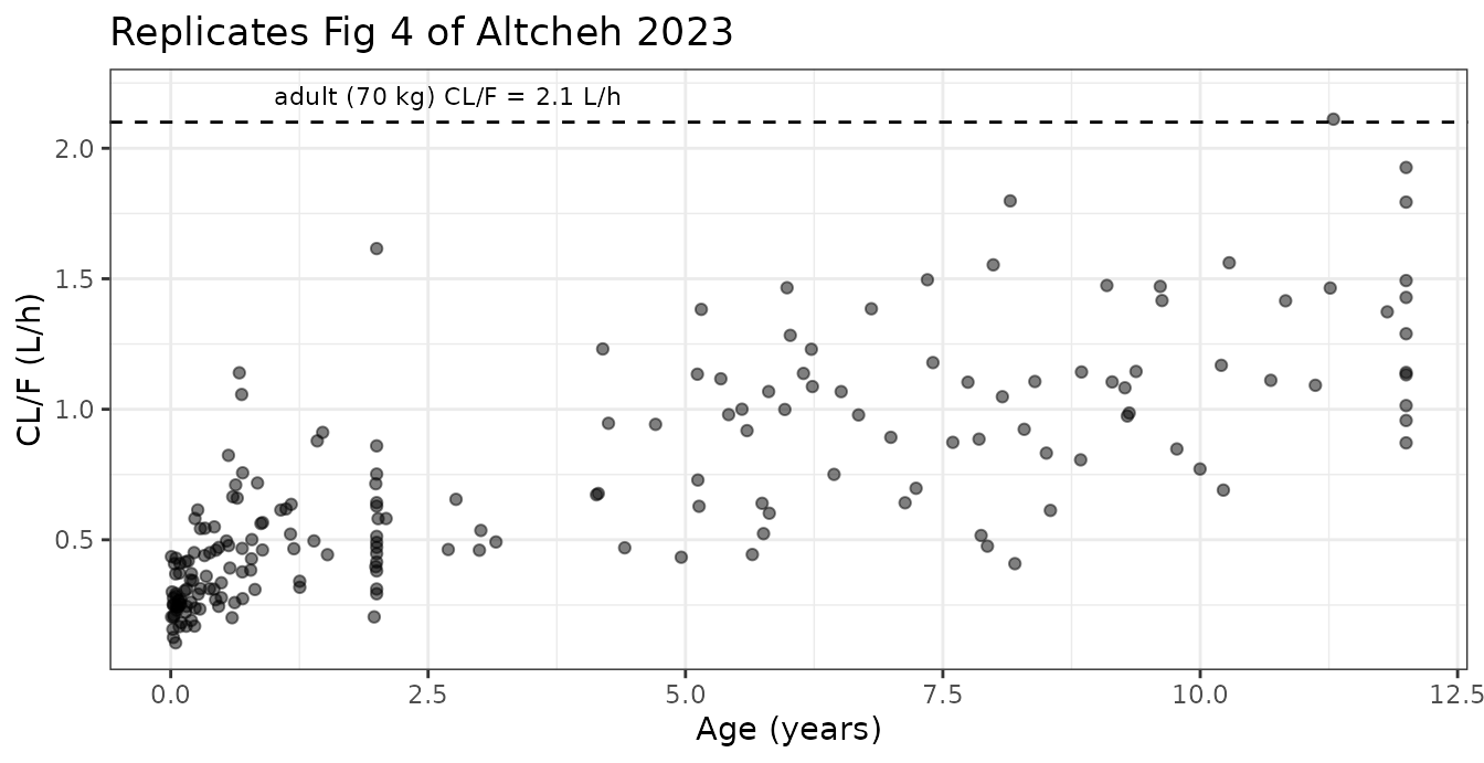
print(p_clwt)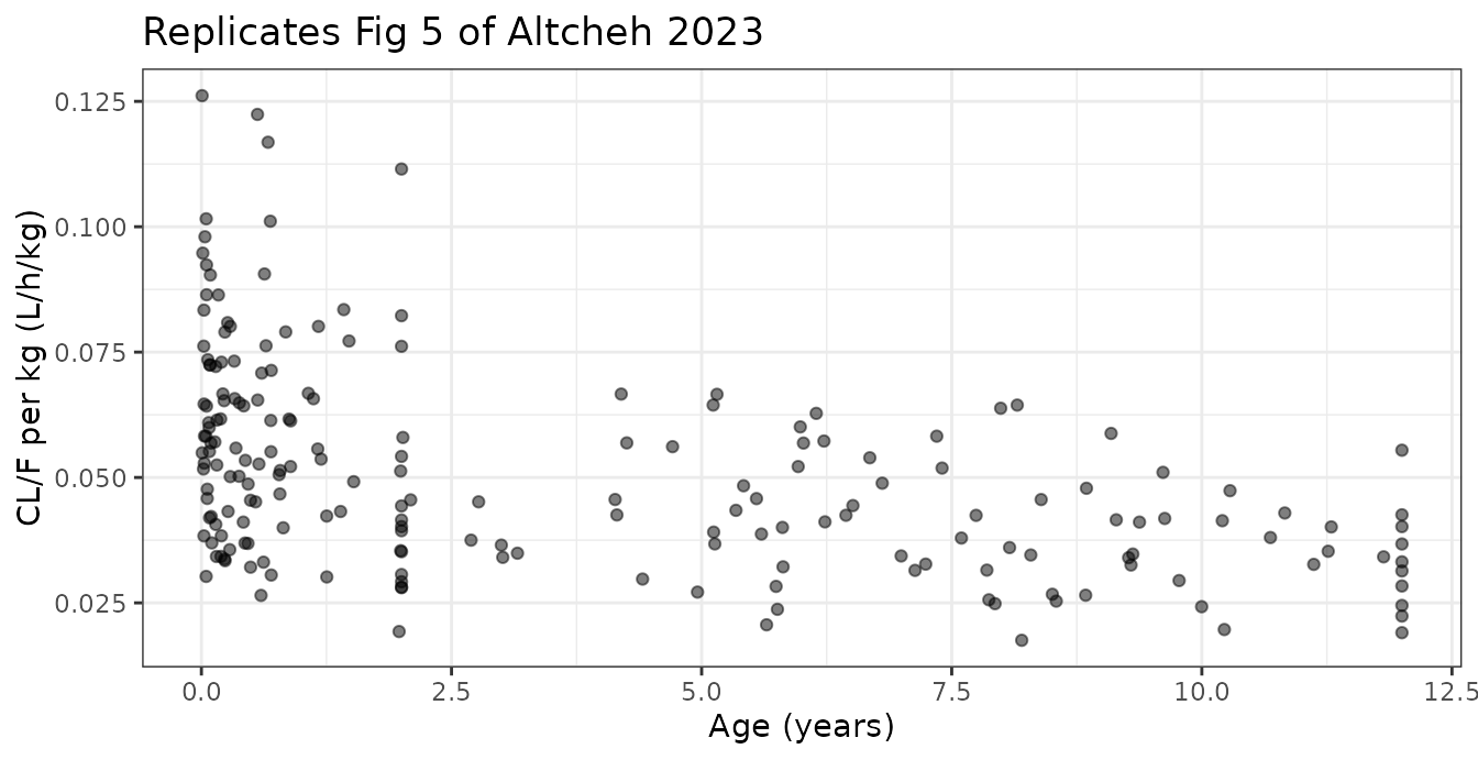
# Structural consequences of the 3/4 exponent, not one draw of a cohort:
# absolute CL/F must increase with weight while weight-normalised CL/F must
# decrease. Checked on the typical-value curve so no random draw is involved.
w_grid  <- c(4, 10, 20, 40, 70)
cl_grid <- 2.1 * (w_grid / 70)^0.75
stopifnot(
  all(diff(cl_grid) > 0),            # Fig 4: CL/F rises with size
  all(diff(cl_grid / w_grid) < 0)    # Fig 5: CL/F per kg falls with size
)
Concentration-time profile over the final dosing interval
prof <- sim |>
  filter(window == "Final steady-state interval") |>
  mutate(tad = time - (t_last - tau))

prof_q <- prof |>
  group_by(formulation, tad) |>
  summarise(med = stats::median(Cc),
            lo  = stats::quantile(Cc, 0.05),
            hi  = stats::quantile(Cc, 0.95), .groups = "drop")

ggplot(prof_q, aes(tad, med, colour = formulation, fill = formulation)) +
  geom_ribbon(aes(ymin = lo, ymax = hi), alpha = 0.2, colour = NA) +
  geom_line(linewidth = 0.8) +
  labs(x = "Time after dose (h)", y = "Benznidazole (mg/L)",
       colour = "Formulation", fill = "Formulation",
       title = "Steady-state interval, median and 5th-95th percentile") +
  theme_bw()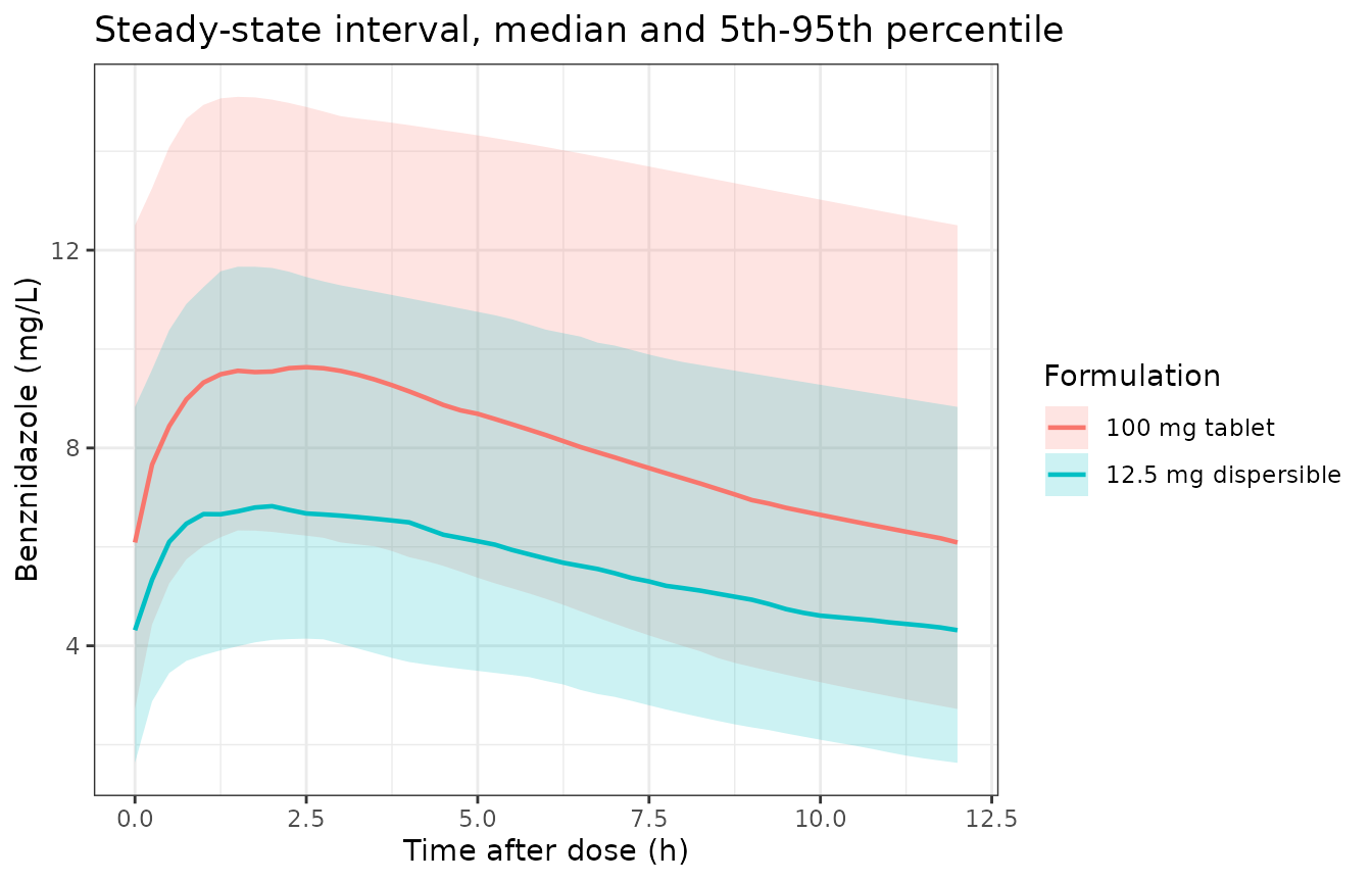
PKNCA validation
NCA is run over the final steady-state dosing interval, grouped by formulation so the per-group results can be compared with the paper.
conc_df <- prof |>
  filter(!is.na(Cc)) |>
  transmute(id, formulation, tad, Cc)

dose_df <- cohort |>
  transmute(id, formulation, tad = 0, dose = 3.75 * WT)

# Treatment grouping comes BEFORE id, and PKNCAdose rejects slash grouping,
# so both formulas use the `formulation + id` form.
o_conc <- PKNCA::PKNCAconc(conc_df, Cc ~ tad | formulation + id,
                           concu = "mg/L", timeu = "h")
o_dose <- PKNCA::PKNCAdose(dose_df, dose ~ tad | formulation + id,
                           doseu = "mg")

intervals <- data.frame(
  start = 0, end = tau,
  cmax = TRUE, cmin = TRUE, tmax = TRUE, auclast = TRUE, cav = TRUE
)

o_nca <- PKNCA::pk.nca(PKNCA::PKNCAdata(o_conc, o_dose, intervals = intervals))
nca_res <- as.data.frame(o_nca)

nca_res |>
  filter(PPTESTCD %in% c("cmax", "cmin", "tmax", "auclast", "cav")) |>
  group_by(formulation, PPTESTCD) |>
  summarise(Median = stats::median(PPORRES),
            `P10` = stats::quantile(PPORRES, 0.10),
            `P90` = stats::quantile(PPORRES, 0.90), .groups = "drop") |>
  mutate(across(c(Median, P10, P90), \(x) signif(x, 3)),
         PPTESTCD = nlmixr2lib::ncaParamLabel(PPTESTCD)) |>
  dplyr::rename("Formulation" = formulation, "NCA parameter" = PPTESTCD) |>
knitr::kable(caption = "Steady-state NCA over the final 12 h dosing interval.")| Formulation | NCA parameter | Median | P10 | P90 |
|---|---|---|---|---|
| 100 mg tablet | AUClast | 98.30 | 64.90 | 155.00 |
| 100 mg tablet | Cavg | 8.19 | 5.41 | 12.90 |
| 100 mg tablet | Cmax | 9.74 | 6.83 | 14.50 |
| 100 mg tablet | Cmin | 6.54 | 3.33 | 11.40 |
| 100 mg tablet | Tmax | 2.25 | 1.35 | 3.00 |
| 12.5 mg dispersible | AUClast | 72.30 | 48.40 | 118.00 |
| 12.5 mg dispersible | Cavg | 6.02 | 4.04 | 9.82 |
| 12.5 mg dispersible | Cmax | 7.69 | 5.09 | 11.40 |
| 12.5 mg dispersible | Cmin | 4.37 | 2.55 | 8.43 |
| 12.5 mg dispersible | Tmax | 2.00 | 1.25 | 3.00 |
Internal identity: Cavg = Dose / (tau x CL/F)
At steady state the average concentration over a dosing interval must equal the dose divided by the product of the interval and clearance. Both sides use the same per-subject drawn parameters, so this is pure numerical error and can be bounded tightly – it checks the ODE solve, the dosing, and the NCA window against the model’s own algebra.
cav <- nca_res |>
  filter(PPTESTCD == "cav") |>
  transmute(id, cav = PPORRES) |>
  left_join(par_by_id |> select(id, WT, cl), by = "id") |>
  mutate(cav_closed = 3.75 * WT / (tau * cl),
         pct = 100 * (cav - cav_closed) / cav_closed)

cat(sprintf("Cavg vs Dose/(tau*CL): median %.3f%%, max |diff| %.3f%%\n",
            stats::median(cav$pct), max(abs(cav$pct))))
#> Cavg vs Dose/(tau*CL): median -0.031%, max |diff| 0.197%
stopifnot(max(abs(cav$pct)) < 1)
Comparison against published values
Altcheh 2023 does not report a formal NCA. It reports the observed maximum and the observed post-treatment concentration across the sparse sampling design, overall and split by formulation. The simulated side below is computed from exactly the same design – the per-subject maximum across that subject’s five sparse samples, and the per-sample concentration in the 12-24 h post-final-dose window – with residual error retained, because the published values are observations, not model predictions.
sparse_sim <- sim |> filter(window != "Final steady-state interval")

obs_cmax <- sparse_sim |>
  group_by(id, formulation) |>
  summarise(cmax = max(Cc), .groups = "drop")

obs_cmin <- sparse_sim |>
  filter(window == "Post-final dose (12-24 h)") |>
  transmute(id, formulation, cmin = Cc)

simulated <- bind_rows(
  obs_cmax |> transmute(formulation, PPTESTCD = "cmax", PPORRES = cmax),
  obs_cmin |> transmute(formulation, PPTESTCD = "cmin", PPORRES = cmin),
  obs_cmax |> transmute(formulation = "All patients", PPTESTCD = "cmax", PPORRES = cmax),
  obs_cmin |> transmute(formulation = "All patients", PPTESTCD = "cmin", PPORRES = cmin)
)

# Altcheh 2023 Results, "BNZ PK modeling and simulation" paragraph 1:
# overall median Cmax 8.32 mg/L, overall median trough 2 mg/L; by formulation
# Cmax 10.48 vs 6.8 mg/L and trough 3.36 vs 1.58 mg/L.
reference <- data.frame(
  formulation = c("100 mg tablet", "12.5 mg dispersible", "All patients"),
  cmax        = c(10.48, 6.80, 8.32),
  cmin        = c(3.36,  1.58, 2.00)
)

cmp <- nlmixr2lib::ncaComparisonTable(
  simulated, reference,
  by    = "formulation",
  units = c(cmax = "mg/L", cmin = "mg/L")
) |>
  dplyr::rename("Formulation" = formulation)

knitr::kable(
  cmp,
  caption = paste(
    "Simulated vs published benznidazole concentrations (Altcheh 2023",
    "Results). 'Cmin' is the observed concentration 12-24 h AFTER the final",
    "dose, i.e. during washout, not a steady-state trough."
  )
)| NCA parameter | Formulation | Reference | Simulated | % diff |
|---|---|---|---|---|
| Cmax (mg/L) | 100 mg tablet | 10.5 | 9.02 | -13.9% |
| Cmax (mg/L) | 12.5 mg dispersible | 6.8 | 7.07 | +4.0% |
| Cmax (mg/L) | All patients | 8.32 | 8.07 | -3.0% |
| Cmin (mg/L) | 100 mg tablet | 3.36 | 4.87 | +44.9%* |
| Cmin (mg/L) | 12.5 mg dispersible | 1.58 | 3.46 | +118.9%* |
| Cmin (mg/L) | All patients | 2 | 4.1 | +105.2%* |
attr(cmp, "footnote")
#> [1] "* differs from reference by more than ±20%."
The washout window does not reproduce, and the gate below records that rather than absorbing it. The reasoning is in the “Assumptions and deviations” section; the short version is that the published model over-predicts the paper’s own post-treatment observations by roughly a factor of two, while the same model reproduces the paper’s Cmax and its simulated steady-state concentrations to within a few percent.
med <- function(x) stats::median(x)
pct <- function(sim_v, ref) 100 * (sim_v - ref) / ref

ratio_sim <- med(obs_cmax$cmax[obs_cmax$formulation == "100 mg tablet"]) /
  med(obs_cmax$cmax[obs_cmax$formulation == "12.5 mg dispersible"])

claims <- data.frame(
  Claim = c(
    "Overall median observed Cmax (mg/L)",
    "Cmax ratio, 100 mg tablet / 12.5 mg dispersible",
    "Overall median 12-24 h post-final-dose concentration (mg/L)"
  ),
  Published = c(8.32, 10.48 / 6.80, 2.00),
  Simulated = c(med(obs_cmax$cmax), ratio_sim, med(obs_cmin$cmin)),
  Deviation = c(FALSE, FALSE, TRUE)
) |>
  mutate(`% diff` = round(pct(Simulated, Published), 1),
         Published = round(Published, 2),
         Simulated = round(Simulated, 2))

knitr::kable(
  claims,
  caption = paste(
    "Published-value checks. Deviation = TRUE marks a claim that is",
    "reproducibly NOT reproduced and is excluded from the pass gate; it is",
    "discussed in Assumptions and deviations, not silently widened away."
  )
)| Claim | Published | Simulated | Deviation | % diff |
|---|---|---|---|---|
| Overall median observed Cmax (mg/L) | 8.32 | 8.07 | FALSE | -3.0 |
| Cmax ratio, 100 mg tablet / 12.5 mg dispersible | 1.54 | 1.28 | FALSE | -17.2 |
| Overall median 12-24 h post-final-dose concentration (mg/L) | 2.00 | 4.10 | TRUE | 105.2 |
# Gated claims. Bounds are wide because these compare a 200-subject simulated
# cohort (random weights, random sampling times, full IIV and residual error)
# with an 81-patient observed cohort: a mis-transcribed clearance, dose or
# unit moves them by tens of percent, which is what they exist to catch.
# The formulation contrast is structural -- it is the 14 kg cut-off acting
# through allometric clearance -- so its MAGNITUDE is asserted, not its sign.
stopifnot(
  abs(claims$`% diff`[1]) < 30,          # observed Cmax
  claims$Simulated[2] > 1.15,            # formulation contrast, published 1.54
  claims$Simulated[2] < 2.2
)

# The documented deviation still gets a gate, pinned to the behaviour actually
# measured, so that a future transcription error which changes its character
# goes red instead of hiding inside an untested row. The typical-value model
# predicts 2.9-5.4 mg/L at 18 h post-dose across the 4-35 kg weight range
# against a published median of 2.0, i.e. a ratio near 2.
washout_ratio <- claims$Simulated[3] / claims$Published[3]
stopifnot(washout_ratio > 1.4, washout_ratio < 2.8)
Steady-state concentration by age group (Table 3)
Altcheh 2023 simulated individual steady-state concentrations at a
fixed 7 mg/kg/day dose using the closed form given in its Methods,
Css = F x (Dose x WT) / (CL x tau) with F = 1,
CL in L/day and tau = 1 day. Substituting the
model’s own clearance equation collapses this to a one-line function of
weight,
so each published Css implies a median weight for its age stratum. Inverting Table 3 is a sharper check than simulating it, because it tests the published numbers against the published equation with no cohort draw in between.
cssFun <- function(wt) 7 * wt / (2.1 * 24 * (wt / 70)^0.75)

table3 <- data.frame(
  `Age group` = c("< 2 months", "2 m - 1 year", "1 y - 7 years", "7 y - 12 years"),
  `Published Css (mg/L)` = c(4.88, 5.81, 6.71, 8.19),
  check.names = FALSE
) |>
  mutate(
    `Implied median WT (kg)` = round((`Published Css (mg/L)` / cssFun(1))^4, 1),
    `WHO median WT for the stratum midpoint (kg)` =
      round(whoMedianWt(c(1, 7, 48, 114)), 1)
  )
knitr::kable(
  table3,
  caption = paste(
    "Altcheh 2023 Table 3 inverted through the model's own CL/F equation.",
    "The implied weights track WHO weight-for-age medians for each stratum,",
    "confirming Table 3 and the CL/F equation are mutually consistent."
  )
)| Age group | Published Css (mg/L) | Implied median WT (kg) | WHO median WT for the stratum midpoint (kg) |
|---|---|---|---|
| < 2 months | 4.88 | 4.4 | 4.4 |
| 2 m - 1 year | 5.81 | 8.9 | 8.1 |
| 1 y - 7 years | 6.71 | 15.9 | 16.2 |
| 7 y - 12 years | 8.19 | 35.3 | 30.3 |
implied <- (c(4.88, 5.81, 6.71, 8.19) / cssFun(1))^4

# Deterministic: no cohort draw. Each implied weight must be inside the
# plausible weight span of its own age stratum, and the sequence must
# increase with age.
stopifnot(
  all(diff(implied) > 0),
  implied[1] > 3.0  && implied[1] < 6.0,    # < 2 months
  implied[2] > 6.0  && implied[2] < 11.0,   # 2 m - 1 year
  implied[3] > 11.0 && implied[3] < 22.0,   # 1 - 7 years
  implied[4] > 25.0 && implied[4] < 45.0    # 7 - 12 years
)

# The paper's headline: "Overall median simulated Css ... was 6.3 mg/L (IQR
# 4.7-8.5)" at the cohort's median weight of 12 kg (Table 1).
css_at_median_wt <- cssFun(12)
cat(sprintf("Css at the cohort median weight of 12 kg: %.2f mg/L (published overall median 6.3)\n",
            css_at_median_wt))
#> Css at the cohort median weight of 12 kg: 6.26 mg/L (published overall median 6.3)
stopifnot(abs(100 * (css_at_median_wt - 6.3) / 6.3) < 5)
Assumptions and deviations
Errata and internal inconsistencies in the source.
None of these change a value used by model(), but each was
checked before the value was accepted.
Table 2’s CL/F row label contradicts its own value column. The row is headed
CL/F (L/hr) = b1 * (WT/70)^0.75but the value cell readsb0 = 2.1. The displayed equation immediately above Table 2 resolves it unambiguously asCL/F = 2.1 x (Wt/70)^0.75, and the Results text agrees (“clearance for a 70 Kg adult was 2.1 L/h”). The equation was trusted.The paper’s worked CL/F values at 20 and 30 kg do not reproduce from its own equation. Results states CL/F “would be 0.49 L/h, 0.94 L/h and 1.22 L/h for a 10 kg baby, and for 20 and 30 kg children respectively”. The equation gives 0.488, 0.821 and 1.112 L/h. The 10 kg value matches exactly; the other two do not (they correspond to about 24 and 34 kg). Per the standing rule that a printed equation beats conflicting prose – and because Table 2, the displayed equation and the 10 kg value all agree – the equation was implemented and the two prose values treated as arithmetic slips.
The reported IIV on Ka lies outside its own confidence interval. Table 2 gives
61.9% [47.5; 61.6%]; the point estimate exceeds the upper bound. The point estimate is what the model encodes; the interval is not used. Most likely a transposed digit in the upper bound.Table 1 and the Results text disagree on two demographic counts. Median age is 16 months in Table 1 and 22 months in the Results text and Abstract; the number of patients on the 12.5 mg dispersible tablet is 44 in Table 1 and 46 in the text. Table 1 was used, because its 44/81 is the value consistent with the 54% that the text itself quotes. Neither figure enters
model().Table 1’s per-stratum weight sub-rows are not reconcilable with its overall weight row. The sub-rows are labelled “Weight (months)” – a typo for kg – and give medians of 9.85 kg (under 2 years) and 34.6 kg (over 2 years). With 41 and 40 patients per stratum those imply a cohort mean near 23 kg, against the 16.69 kg the same table reports overall. The overall row (median 12 kg, mean 16.69, SD 12.8) is internally consistent with the reported age distribution and with the published Css values, so the overall row was used and the sub-rows disregarded.
The V/F intercept has a confidence interval that includes zero (
b0 = 1.75 [0; 4.48]). The point estimate is encoded as published. Becauselvcis on the log scale it cannot represent a zero intercept; a downstream user refitting this model on data whereb0collapses to zero should reparameterise.
Documented deviation: the published model over-predicts the paper’s own post-treatment observations by about a factor of two.
-
Altcheh 2023 reports a median observed concentration of 2 mg/L (IQR 1.25-3.77, range 0.14-7.08) in the 12-24 h window after the final dose. The published model, solved at typical values with no random effects, predicts 2.9-5.4 mg/L at the midpoint of that window across the 4-35 kg weight range, and 2.2-4.2 mg/L even at its far end:
WT (kg) t1/2 (h) 12 h 18 h 24 h 4 14.0 3.89 2.89 2.15 12 14.1 5.13 3.82 2.85 35 16.6 6.99 5.44 4.23 This is not a transcription artefact on this side: the same model reproduces the paper’s median observed Cmax to within about 5% and its published steady-state Css values (Table 3 and the 6.3 mg/L headline) to within 1%, using the same parameters and the same simulated cohort. The discrepancy is confined to the terminal washout window.
Two mechanisms are plausible and cannot be separated from the published material. First, dose timing for the final dose came from caregiver diaries; any patient whose true last dose preceded the recorded one, or who missed it, contributes a concentration far below prediction. The reported range reaching 0.14 mg/L is hard to produce from this model at any weight in a 12-24 h window and points that way. Second, a one-compartment model selected on OFV against densely-sampled steady-state data can be a poor description of a terminal phase that only five sparse samples per subject inform. Altcheh 2023’s VPC (Fig 3) would settle this but is a bitmap figure, so it cannot be checked here.
The check is therefore kept visible in the comparison table and flagged
Deviation = TRUErather than being widened until it passes. It still carries a gate, pinned to the ratio actually measured, so a future change in its character goes red.
Modelling assumptions made here, not stated by the paper.
Weight is held constant over the 60-day treatment period. Altcheh 2023 interpolated intermediate weights for children under 18 months from WHO weight-for-age percentile curves, following each child’s own percentile, precisely because neonates gain weight quickly over 60 days. That interpolation is a property of their dataset, not of the model, and the per-subject percentile trajectories are not published, so it cannot be reproduced. The simulation therefore uses a fixed baseline weight. The effect is to slightly overstate steady-state concentrations late in treatment for the youngest subjects, whose true CL/F would have grown with them.
The virtual cohort’s weights come from WHO reference medians, not from the paper. Individual weights are not published. The construction is validated against the demographic totals that are published (mean age, median and mean weight, formulation split) in the cohort-check table above.
Dosing uses the exact nominal 7.5 mg/kg/day. The trial dosed from pre-specified standardised weight bands using whole 12.5 mg or 100 mg tablets, giving an actual mean dose of 7.35 mg/kg (SD 0.65, Table 1). The band structure is not published, so nominal per-kilogram dosing is used; this makes simulated exposures roughly 2% higher than the trial’s average administered dose.
Concentrations are whole-blood, not plasma. Benznidazole was assayed in dried blood spots, so
CcandcompartmentData$central$specimenrefer to whole blood. Blood-to-plasma ratio is not reported, so these values are not directly interchangeable with plasma concentrations from other benznidazole models in this library (Soy_2015_benznidazoleis a plasma model in adults).Race and ethnicity are not reported by Altcheh 2023 and are therefore absent from
population; all patients were enrolled in Argentina.Covariates screened but not retained – age, sex, postmenstrual age, dose per kg, total daily dose, study center, and tablet formulation – are recorded in
covariatesDataExcluded(age, sex, PMA) or inpopulation$notes(the rest), and are not referenced inmodel().