Atazanavir (Foissac 2011)
Source:vignettes/articles/Foissac_2011_atazanavir.Rmd
Foissac_2011_atazanavir.RmdModel and source
- Citation: Foissac F, Blanche S, Dollfus C, Hirt D, Firtion G, Laurent C, Treluyer JM, Urien S. Population pharmacokinetics of atazanavir/ritonavir in HIV-1-infected children and adolescents. Br J Clin Pharmacol. 2011;72(6):940-947. doi:10.1111/j.1365-2125.2011.04035.x.
- Description: One-compartment first-order-absorption population PK model for orally administered atazanavir in 51 HIV-1-infected children and adolescents (3-18 years, 13-79 kg) on therapeutic drug monitoring. Body weight is carried through a fixed-exponent allometric scaling on CL/F (0.75) and V/F (1.0) referenced to 70 kg. Two binary co-medication indicators enter linearly on apparent oral clearance: low-dose ritonavir as a PK booster reduces CL/F (the typical CL/F = 7.1 L/h is the RTV-boosted reference, and absence of ritonavir multiplies CL/F by 1.80) and concomitant 300 mg tenofovir disoproxil fumarate increases CL/F by 25%. Between-subject variability is retained only on CL/F; residual error is proportional (Foissac 2011).
- Article: Br J Clin Pharmacol. 2011;72(6):940-947
Foissac et al. (2011) describe a one-compartment first-order-absorption population PK model for orally administered atazanavir in 51 HIV-1-infected children and adolescents (3-18 years, body weight 13-79 kg) on routine therapeutic drug monitoring. Body weight is carried through a fixed-exponent allometric scaling on CL/F (0.75) and V/F (1.0) referenced to 70 kg. Two binary co-medication indicators retained in the final model enter linearly on apparent oral clearance: low-dose ritonavir as a PK booster reduces CL/F (the typical CL/F = 7.1 L/h is the RTV-boosted reference, and absence of ritonavir multiplies CL/F by 1.80), and concomitant 300 mg tenofovir disoproxil fumarate (TDF) increases CL/F by 25%. Between-subject variability is retained only on CL/F (BSV = 0.16); residual error is proportional (53% CV).
Population
The model-building cohort is 51 HIV-1-infected children (25 girls, 26 boys) followed at four Assistance Publique Hopitaux de Paris hospitals (Necker, Trousseau, Cochin/Saint-Vincent-de-Paul, Louis Mourier) on routine therapeutic drug monitoring (Foissac 2011 Table 1). Median age 14 years (range 3-18 years), median body weight 52 kg (range 13-79 kg). 39 children received boosted atazanavir/ritonavir (ATV/r), 9 received unboosted atazanavir, and 3 received both regimens successively; 21 of the 39 ATV/r-treated children additionally received tenofovir disoproxil fumarate at 300 mg q.d. (median 300 mg, range 150-300 mg). Median ATV/r and ATV doses were 300/100 mg and 400 mg respectively (ATV/r 100-400 mg, ATV 150-600 mg). 151 ATV plasma concentrations were available across the 51 subjects (median 2 samples per patient, range 1-13) over a median 2.3-month follow-up (range 0-34 months). Atazanavir was assayed by HPLC with LOQ = 0.10 mg/L; four BLQ observations (< 3% of the dataset) were handled by setting them to LOQ/2. The model was fit with NONMEM VI under FOCE-INTERACTION and validated by 1000 bootstrap analyses (Wings for Nonmem) plus visual predictive checks and normalized prediction distribution errors.
The same information is available programmatically via the model’s
population metadata
(readModelDb("Foissac_2011_atazanavir")$population).
Source trace
The per-parameter origin is recorded as an in-file comment next to
each ini() entry in
inst/modeldb/specificDrugs/Foissac_2011_atazanavir.R. The
table below collects them in one place for review.
| Parameter | Value | Source location |
|---|---|---|
lcl |
log(7.1) |
Table 2: CL/F = 7.1 L/h (70 kg)^-1 at CONMED_RTV = 1, CONMED_TDF = 0 (RSE 8%) |
lvc |
log(103) |
Table 2: V/F = 103 L (70 kg)^-1 (RSE 19%) |
lka |
log(0.44) |
Table 2: Ka = 0.44 1/h (RSE 26%) |
allo_cl |
fixed(0.75) |
Methods: PWR = 0.75 for CL (FIXED at allometric-theory value) |
allo_v |
fixed(1) |
Methods: PWR = 1 for V (FIXED at allometric-theory value) |
e_no_rtv_cl |
0.80 |
Table 2: theta_NO_RTV (CL/F) = 0.80 (RSE 24%) |
e_tdf_cl |
0.25 |
Table 2: theta_TDF (CL/F) = 0.25 (RSE 37%) |
etalcl |
0.16^2 |
Table 2: BSV(CL/F) = 0.16 (sqrt of omega; RSE 34%); variance = 0.0256 |
propSd |
0.53 |
Table 2: sigma_proportional = 0.53 (RSE 15%) |
Covariate equation (Foissac 2011 Table 2 footnote):
CL/F_i = exp(lcl + etalcl_i)
       * (1 + e_no_rtv_cl * (1 - CONMED_RTV_i))
       * (1 + e_tdf_cl    * CONMED_TDF_i)
       * (WT_i / 70)^allo_cl
V/F_i  = exp(lvc) * (WT_i / 70)^allo_v
where CONMED_RTV = 1 is the boosted reference stratum
(typical CL/F = 7.1 L/h at 70 kg), CONMED_RTV = 0 flips on
the theta_NO_RTV effect (CL/F multiplied by 1.80 -> 12.8
L/h at 70 kg per Table 2 footnote), and CONMED_TDF = 1 adds
a further 25% increase (giving 8.9 L/h at 70 kg under ATV/r + TDF, again
matching the Table 2 footnote arithmetic).
ODE structure: one-compartment first-order absorption from
depot to central. The observation variable is
Cc = central / vc (dose in mg, V in L give Cc in mg/L).
Residual error is proportional only.
Load model
mod         <- readModelDb("Foissac_2011_atazanavir")
mod_typical <- rxode2::zeroRe(mod)
#> ℹ parameter labels from comments will be replaced by 'label()'
Typical-value steady-state profiles (three regimens)
The block below reproduces the typical-value 14-day steady-state profile for the three regimens that Foissac 2011 explicitly discusses (Table 2 footnote and Discussion paragraph 1):
- 400 mg q.d. unboosted atazanavir (
CONMED_RTV = 0,CONMED_TDF = 0): typical CL/F at 70 kg is7.1 * 1.80 = 12.8 L/h. - 300/100 mg q.d. ATV/r without TDF (
CONMED_RTV = 1,CONMED_TDF = 0): typical CL/F at 70 kg is7.1 L/h. - 300/100 mg q.d. ATV/r with 300 mg TDF (
CONMED_RTV = 1,CONMED_TDF = 1): typical CL/F at 70 kg is7.1 * 1.25 = 8.9 L/h.
n_doses <- 14L   # 14 once-daily doses to approach steady state
ii      <- 24    # h

make_typical_events <- function(id, amt, rtv, tdf) {
  dose_times <- (seq_len(n_doses) - 1L) * ii
  obs_times  <- seq(0, n_doses * ii, by = 0.5)
  ev <- data.frame(
    id   = id,
    time = c(dose_times, obs_times),
    amt  = c(rep(amt, length(dose_times)), rep(0,  length(obs_times))),
    evid = c(rep(1L,   length(dose_times)), rep(0L, length(obs_times))),
    cmt  = c(rep("depot", length(dose_times)),
             rep("central", length(obs_times)))
  )
  ev <- ev[order(ev$id, ev$time, -ev$evid), ]
  ev$WT         <- 70
  ev$CONMED_RTV <- rtv
  ev$CONMED_TDF <- tdf
  ev
}

ev_typ <- dplyr::bind_rows(
  make_typical_events(id = 1L, amt = 400, rtv = 0L, tdf = 0L),
  make_typical_events(id = 2L, amt = 300, rtv = 1L, tdf = 0L),
  make_typical_events(id = 3L, amt = 300, rtv = 1L, tdf = 1L)
)

ev_typ$regimen <- factor(
  paste0(ev_typ$id),
  levels = c("1", "2", "3"),
  labels = c(
    "400 mg ATV q.d. (unboosted)",
    "300/100 mg ATV/r q.d. (no TDF)",
    "300/100 mg ATV/r + 300 mg TDF q.d."
  )
)

sim_typ <- as.data.frame(
  rxode2::rxSolve(mod_typical, ev_typ,
                  keep = c("regimen", "CONMED_RTV", "CONMED_TDF", "WT"))
)
#> ℹ omega/sigma items treated as zero: 'etalcl'
#> Warning: multi-subject simulation without without 'omega'

ggplot(sim_typ, aes(time / 24, 1000 * Cc, colour = regimen)) +
  geom_line(linewidth = 0.6) +
  labs(
    x        = "Time (days)",
    y        = "Atazanavir concentration (ng/mL)",
    colour   = "Regimen",
    title    = "Typical-value 14-day steady-state atazanavir profiles (WT = 70 kg)"
  ) +
  theme_bw() +
  theme(legend.position = "bottom", legend.direction = "vertical")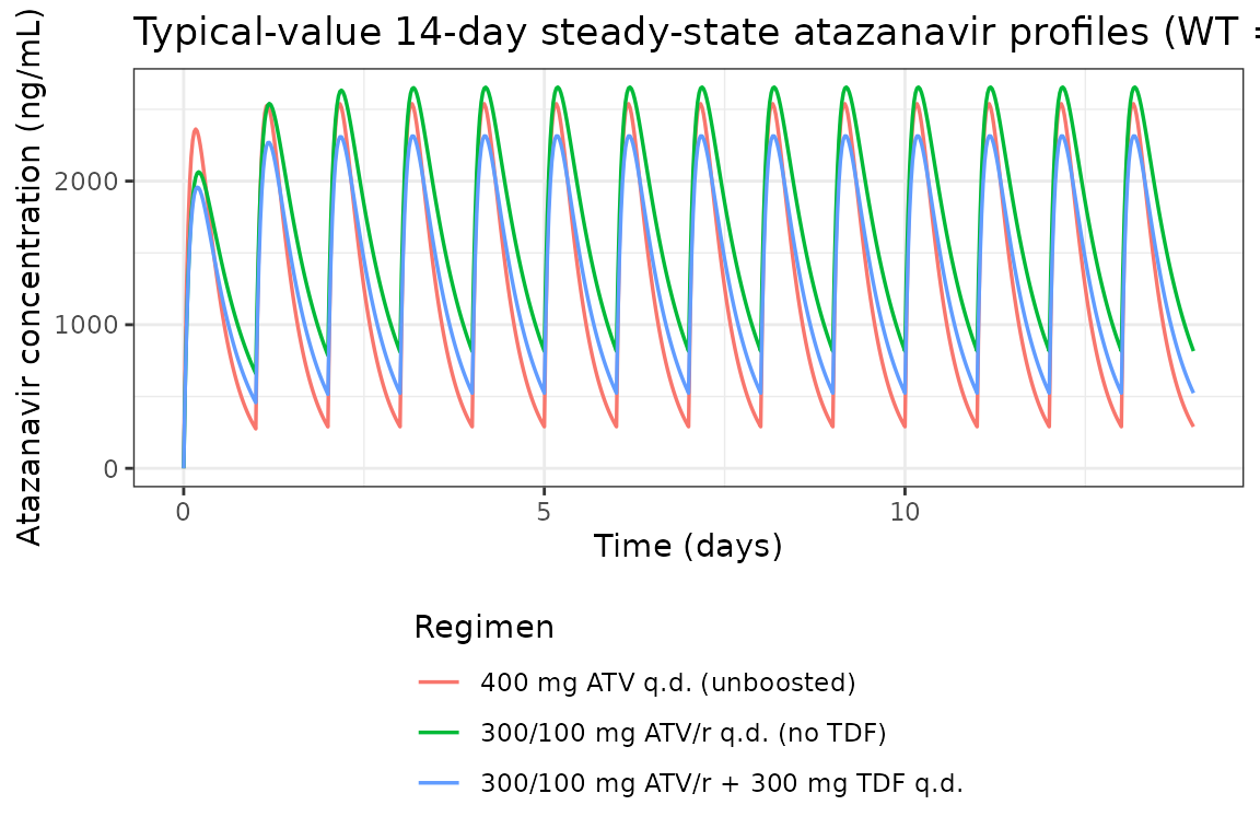
Steady-state dosing interval (Day 14)
sim_tau <- sim_typ |>
  dplyr::filter(time >= 13 * 24, time <= 14 * 24) |>
  dplyr::mutate(t_post_dose = time - 13 * 24)

ggplot(sim_tau, aes(t_post_dose, 1000 * Cc, colour = regimen)) +
  geom_line(linewidth = 0.7) +
  labs(
    x       = "Time after dose (h)",
    y       = "Atazanavir concentration (ng/mL)",
    colour  = "Regimen",
    title   = "Typical-value Day-14 steady-state dosing interval (WT = 70 kg)"
  ) +
  theme_bw() +
  theme(legend.position = "bottom", legend.direction = "vertical")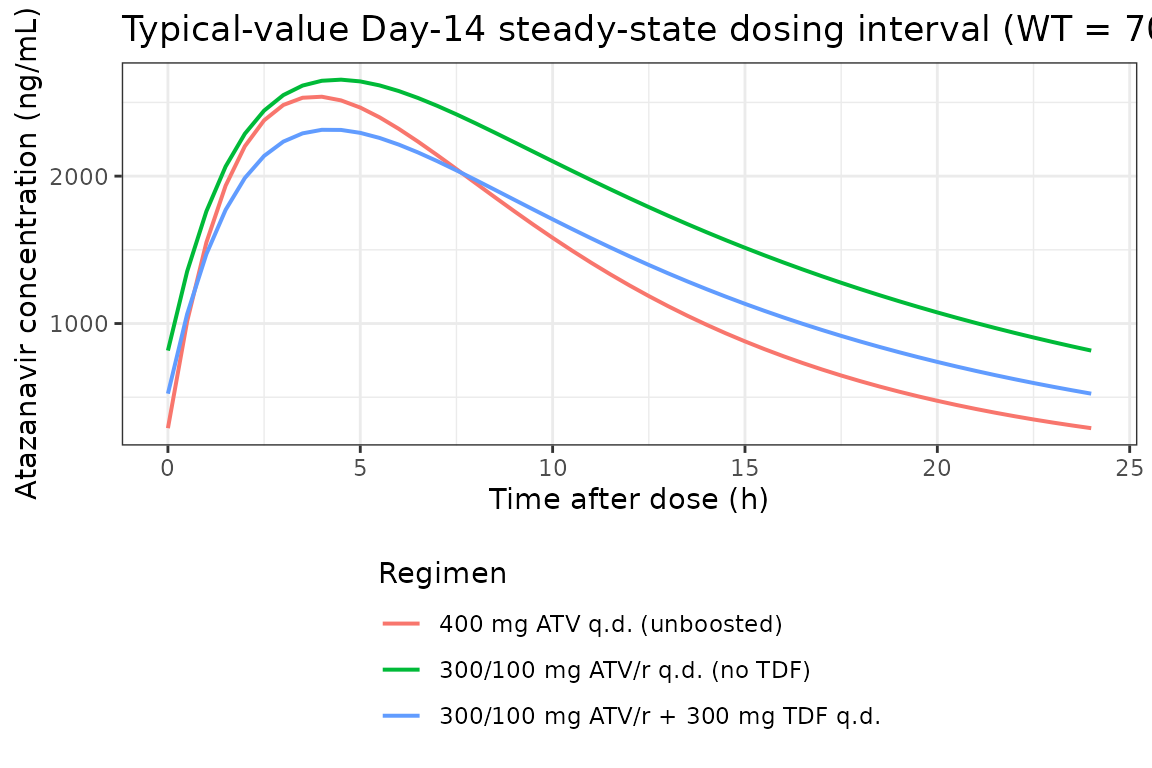
Virtual cohort matched to study demographics
We build a virtual paediatric cohort that reflects the Foissac 2011 cohort proportions: 30 ATV/r-without-TDF subjects, 21 ATV/r-with-TDF subjects, and 9 ATV-alone subjects (the 3 children who received both ATV-alone and ATV/r successively are not separately modelled here; they are absorbed into the larger ATV/r stratum). Body weights are drawn from a normal distribution matched to Table 1 mean (51 kg) and SD (15 kg), truncated to the published range 13-79 kg.
set.seed(2011)

draw_wt <- function(n, mean_wt = 51, sd_wt = 15, lo = 13, hi = 79) {
  pmin(pmax(rnorm(n, mean = mean_wt, sd = sd_wt), lo), hi)
}

make_cohort <- function(n, regimen_label, amt, rtv, tdf, id_offset = 0L) {
  ids        <- id_offset + seq_len(n)
  wt_subject <- draw_wt(n)
  dose_times <- (seq_len(n_doses) - 1L) * ii
  obs_times  <- c(seq(0, ii, by = 1), seq(13 * ii, 14 * ii, by = 1))

  dose_rows <- data.frame(
    id   = rep(ids, each = length(dose_times)),
    time = rep(dose_times, times = n),
    amt  = amt,
    evid = 1L,
    cmt  = "depot",
    WT   = rep(wt_subject, each = length(dose_times))
  )

  obs_rows <- data.frame(
    id   = rep(ids, each = length(obs_times)),
    time = rep(obs_times, times = n),
    amt  = 0,
    evid = 0L,
    cmt  = "central",
    WT   = rep(wt_subject, each = length(obs_times))
  )

  ev <- rbind(dose_rows, obs_rows)
  ev <- ev[order(ev$id, ev$time, -ev$evid), ]
  ev$CONMED_RTV <- rtv
  ev$CONMED_TDF <- tdf
  ev$regimen    <- regimen_label
  ev
}

events <- dplyr::bind_rows(
  make_cohort(30L, "300/100 mg ATV/r q.d. (no TDF)",
              amt = 300, rtv = 1L, tdf = 0L, id_offset =  0L),
  make_cohort(21L, "300/100 mg ATV/r + 300 mg TDF q.d.",
              amt = 300, rtv = 1L, tdf = 1L, id_offset = 30L),
  make_cohort( 9L, "400 mg ATV q.d. (unboosted)",
              amt = 400, rtv = 0L, tdf = 0L, id_offset = 51L)
)

# Guard against accidental cross-cohort ID collision
stopifnot(!anyDuplicated(unique(events[, c("id", "time", "evid")])))
Stochastic simulation across the virtual cohort
sim_pop <- rxode2::rxSolve(
  mod, events = events,
  keep = c("regimen", "CONMED_RTV", "CONMED_TDF", "WT")
)
#> ℹ parameter labels from comments will be replaced by 'label()'
sim_pop_df <- as.data.frame(sim_pop)
VPC: Day-1 and Day-14 dosing intervals by regimen
quantile_band <- function(df, time_col) {
  df |>
    dplyr::group_by(.data[[time_col]], regimen) |>
    dplyr::summarise(
      Q05 = quantile(Cc, 0.05, na.rm = TRUE),
      Q50 = quantile(Cc, 0.50, na.rm = TRUE),
      Q95 = quantile(Cc, 0.95, na.rm = TRUE),
      .groups = "drop"
    ) |>
    dplyr::rename(time = !!time_col)
}

sim_day1 <- sim_pop_df |>
  dplyr::filter(time >= 0, time <= ii) |>
  quantile_band("time") |>
  dplyr::mutate(panel = "Day 1")

sim_day14 <- sim_pop_df |>
  dplyr::filter(time >= 13 * ii, time <= 14 * ii) |>
  dplyr::mutate(t_interval = time - 13 * ii) |>
  quantile_band("t_interval") |>
  dplyr::mutate(panel = "Day 14")

vpc_df <- dplyr::bind_rows(sim_day1, sim_day14)

ggplot(vpc_df, aes(time, 1000 * Q50, colour = regimen, fill = regimen)) +
  geom_ribbon(aes(ymin = 1000 * Q05, ymax = 1000 * Q95),
              alpha = 0.18, colour = NA) +
  geom_line(linewidth = 0.7) +
  facet_wrap(~panel) +
  labs(
    x       = "Time after most recent dose (h)",
    y       = "Atazanavir concentration (ng/mL)",
    colour  = "Regimen",
    fill    = "Regimen",
    title   = "Virtual-cohort VPC by regimen: median + 90% prediction interval",
    caption = "Approximate replication of Foissac 2011 Figure 1 (a) ATV/r and (b) ATV/r + TDF visual predictive checks."
  ) +
  theme_bw() +
  theme(legend.position = "bottom", legend.direction = "vertical")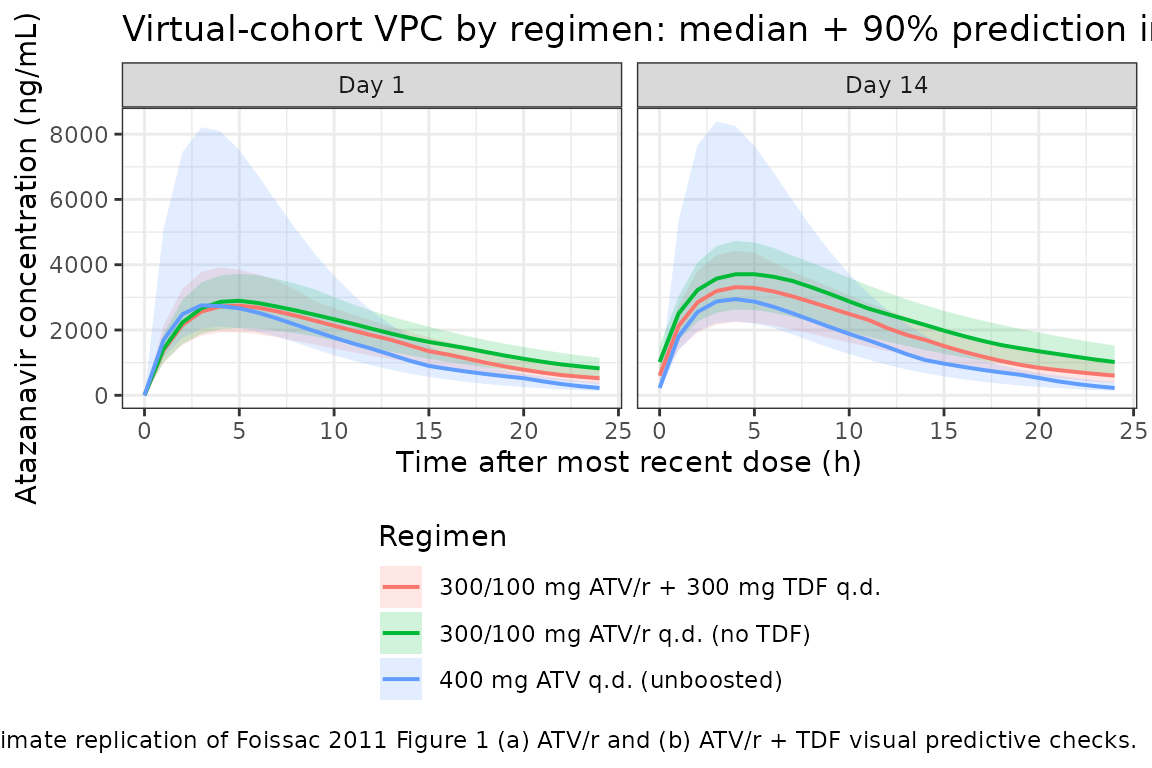
PKNCA validation
Non-compartmental analysis of the simulated Day-14 steady-state dosing interval, by treatment grouping (regimen). The published AUC0-24 reference values for the boosted regimens come from Table 3 of Foissac 2011 (geometric mean across 1000 final-model simulations standardised for a 300/100 mg ATV/r once-daily dose at 70 kg, with or without 300 mg TDF).
nca_concs <- sim_pop_df |>
  dplyr::filter(time >= 13 * ii, time <= 14 * ii) |>
  dplyr::mutate(t_in_interval = time - 13 * ii) |>
  dplyr::filter(!is.na(Cc)) |>
  dplyr::select(id, t_in_interval, Cc, regimen) |>
  dplyr::rename(time = t_in_interval)

# Guarantee a time = 0 row per (id, regimen); for extravascular pre-dose
# Cc = 0 is the correct value.
nca_concs <- dplyr::bind_rows(
  nca_concs,
  nca_concs |> dplyr::distinct(id, regimen) |>
    dplyr::mutate(time = 0, Cc = 0)
) |>
  dplyr::distinct(id, regimen, time, .keep_all = TRUE) |>
  dplyr::arrange(id, regimen, time)

dose_records <- events |>
  dplyr::filter(evid == 1L, time == 13 * ii) |>
  dplyr::mutate(time = 0) |>
  dplyr::select(id, time, amt, regimen)

conc_obj <- PKNCA::PKNCAconc(
  nca_concs, Cc ~ time | regimen + id,
  concu = "mg/L", timeu = "h"
)
dose_obj <- PKNCA::PKNCAdose(
  dose_records, amt ~ time | regimen + id,
  doseu = "mg"
)

intervals <- data.frame(
  start    = 0,
  end      = 24,
  cmax     = TRUE,
  tmax     = TRUE,
  cmin     = TRUE,
  auclast  = TRUE,
  cav      = TRUE
)

nca_data    <- PKNCA::PKNCAdata(conc_obj, dose_obj, intervals = intervals)
nca_results <- PKNCA::pk.nca(nca_data)
nca_df      <- as.data.frame(nca_results$result)

nca_summary <- nca_df |>
  dplyr::filter(PPTESTCD %in% c("cmax", "tmax", "cmin", "auclast", "cav")) |>
  dplyr::group_by(regimen, PPTESTCD) |>
  dplyr::summarise(
    median = median(PPORRES, na.rm = TRUE),
    P05    = quantile(PPORRES, 0.05, na.rm = TRUE),
    P95    = quantile(PPORRES, 0.95, na.rm = TRUE),
    .groups = "drop"
  )

knitr::kable(
  nca_summary,
  digits  = 3,
  caption = "Day-14 steady-state PKNCA summary by regimen (Cc in mg/L; AUC in mg*h/L)"
)| regimen | PPTESTCD | median | P05 | P95 |
|---|---|---|---|---|
| 300/100 mg ATV/r + 300 mg TDF q.d. | auclast | 49.305 | 31.723 | 60.545 |
| 300/100 mg ATV/r + 300 mg TDF q.d. | cav | 2.054 | 1.322 | 2.523 |
| 300/100 mg ATV/r + 300 mg TDF q.d. | cmax | 3.311 | 2.245 | 4.436 |
| 300/100 mg ATV/r + 300 mg TDF q.d. | cmin | 0.601 | 0.371 | 1.021 |
| 300/100 mg ATV/r + 300 mg TDF q.d. | tmax | 4.000 | 4.000 | 4.000 |
| 300/100 mg ATV/r q.d. (no TDF) | auclast | 57.018 | 38.320 | 71.894 |
| 300/100 mg ATV/r q.d. (no TDF) | cav | 2.376 | 1.597 | 2.996 |
| 300/100 mg ATV/r q.d. (no TDF) | cmax | 3.713 | 2.622 | 4.729 |
| 300/100 mg ATV/r q.d. (no TDF) | cmin | 1.020 | 0.574 | 1.524 |
| 300/100 mg ATV/r q.d. (no TDF) | tmax | 4.000 | 4.000 | 5.000 |
| 400 mg ATV q.d. (unboosted) | auclast | 36.956 | 25.861 | 80.721 |
| 400 mg ATV q.d. (unboosted) | cav | 1.540 | 1.078 | 3.363 |
| 400 mg ATV q.d. (unboosted) | cmax | 2.946 | 2.263 | 8.421 |
| 400 mg ATV q.d. (unboosted) | cmin | 0.225 | 0.133 | 0.403 |
| 400 mg ATV q.d. (unboosted) | tmax | 4.000 | 3.000 | 4.000 |
Comparison against published values
Foissac 2011 Table 3 reports geometric means and 95% CIs for ATV/r 300/100 mg once-daily across the 51 paediatric subjects, standardised to 70 kg. The relevant published reference values (geometric means) are:
| Regimen | AUC0-24 (mg*h/L) | Ctrough (mg/L) | Source |
|---|---|---|---|
| ATV/r 300/100 mg q.d. | 41.6 (31.8-51.3) | 0.75 (0.37-1.1) | Table 3 (present-study column) |
| ATV/r 300/100 mg + TDF | 32.8 (25.2-39.1) | 0.47 (0.24-0.74) | Table 3 (present-study column) |
The PKNCA summary above includes the matched simulated medians for the same two regimens; the third row (unboosted 400 mg ATV q.d.) is shown for completeness but is not directly reported in the Foissac 2011 results tables.
For a typical 70 kg subject the model’s algebraic AUC0-24 at steady state is
AUC0-24 = dose / (CL/F)evaluating to 300 / 7.1 = 42.3 mg*h/L under ATV/r
without TDF and 300 / (7.1 * 1.25) = 33.8 mg*h/L under
ATV/r + TDF, both within rounding of the published geometric means (41.6
and 32.8 mg*h/L respectively). The matching steady-state half-lives
are
t_half = ln(2) * V / CL = ln(2) * 103 / 7.1   = 10.1 h    (ATV/r without TDF, 70 kg)
                       = ln(2) * 103 / 8.875  = 8.1 h     (ATV/r + TDF,      70 kg)
                       = ln(2) * 103 / 12.78  = 5.6 h     (unboosted ATV,    70 kg)
ka = 0.44 1/h gives an absorption half-life of
ln(2) / 0.44 = 1.6 h.
Assumptions and deviations
Body-weight distribution for the virtual cohort. Foissac 2011 Table 1 reports the body-weight mean (51 kg) and SD (15 kg) but not the underlying distribution. We draw subject weights from a truncated normal in the published range (13-79 kg); the resulting median sits near the published median (52 kg) without forcing a specific distributional shape on the cohort.
Three children with both ATV-alone and ATV/r episodes are pooled into the ATV/r stratum. The paper reports 39 + 9 + 3 = 51 subjects with three children receiving both regimens successively. Without per-episode timing data we cannot reproduce the cross-over directly, so the virtual cohort is 30 ATV/r-without-TDF + 21 ATV/r-with-TDF + 9 ATV-alone subjects (the three cross-over children are absorbed into the larger ATV/r stratum). This keeps the per-stratum sample sizes representative of the paper’s cohort composition without affecting any structural parameter.
Allometric exponents fixed at theoretical values. The Methods state that the PWR exponents may be estimated but the authors elected to fix them at the allometric-theory values 0.75 for clearance and 1 for volume of distribution. We carry that decision through as
fixed(0.75)andfixed(1)inini()so a downstream user cannot tell whether the values were estimated or held constant without thefixed()wrapper providing that provenance.BSV reported as the square root of the omega estimate. Foissac 2011 Methods state explicitly that the reported BSVs are the square root of omega. Mapped to the nlmixr2 ini() block this means the diagonal variance is BSV^2 (= 0.0256 for CL/F at the published BSV = 0.16). The arithmetic is shown next to the
etalclline in the model file.No IIV on V/F or Ka. The final model retained IIV only on CL/F (Results paragraph 2: “Between-subject variability was retained only for apparent clearance”). Other parameters carry only their typical-value estimates; the model file matches this by omitting
etalvc/etalkafromini().No demographic covariates beyond body weight. Age and sex were screened against pharmacokinetic parameters (Methods paragraph 2) and not retained because the body-weight allometric scaling already removed any residual age effect (Discussion paragraph 2). They are documented in the model file’s
covariatesDataExcludedslot so the provenance is preserved without triggering a convention warning for declared-but-unused covariates.Dosing simulated at q.d. with
addlexpanded to explicit dose rows. The vignette expands the 14-day q.d. dosing schedule to 14 individual dose rows rather than usingaddl, so that each dose can carry the per-subjectWTand the cohort labels without the addl row’s covariate columns being forgotten across repeats.
Reference
- Foissac F, Blanche S, Dollfus C, Hirt D, Firtion G, Laurent C, Treluyer JM, Urien S. Population pharmacokinetics of atazanavir/ritonavir in HIV-1-infected children and adolescents. Br J Clin Pharmacol. 2011;72(6):940-947. doi:10.1111/j.1365-2125.2011.04035.x.