Daptomycin (Balice 2022) • nlmixr2lib

Model and source

Citation: Balice G, Passino C, Bongiorni MG, Segreti L, Russo A, Lastella M, Luci G, Falcone M, Di Paolo A. Daptomycin Population Pharmacokinetics in Patients Affected by Severe Gram-Positive Infections: An Update. Antibiotics (Basel). 2022;11(7):914. doi:10.3390/antibiotics11070914.
Description: One-compartment population PK model with first-order elimination for intravenous daptomycin (30-min infusion, 4-12 mg/kg once daily) in hospitalised adults with severe Gram-positive infections, built from routine therapeutic drug monitoring peak and trough samples (Pisa, Italy; DAPTOLIN study). Clearance is additive-linear in Cockcroft-Gault creatinine clearance centred at 63.35 mL/min with an additive (normal, L/h) between-subject random effect; the volume of distribution is additive-linear in female sex centred at the model-building cohort’s female fraction of 0.309. Residual error is piecewise: an intercept-plus-slope standard deviation (additive + proportional summed linearly) for individual predictions below 80 mg/L and a purely proportional standard deviation at or above 80 mg/L.
Article: https://doi.org/10.3390/antibiotics11070914 (open access)

Balice et al. updated the earlier Di Paolo et al. daptomycin model with routine therapeutic drug monitoring (TDM) data from Pisa University Hospital. The final model is a one-compartment model with first-order elimination, fitted in NONMEM 7.2:

Eq 1: Cl (L/h) = theta1 + theta5 x (ClCr - 63.35) / 100 + eta
Eq 2: Vd (L) = theta2 - theta6 x (Sex - 0.309), with Sex = 0 for males and 1 for females.

Residual error is piecewise. For individual predictions (IPRED) below 80 mg/L the residual SD is an intercept-plus-slope function of the additive and proportional thetas. At or above 80 mg/L it is proportional to a third theta, the “error slope for higher iPRED”.

Population

The final model was estimated on a model-building subset of 94 adults (65 men, 29 women; age 65.7 +/- 13.2 years, weight 72.6 +/- 10.9 kg, Cockcroft-Gault creatinine clearance 74.6 +/- 39.7 mL/min; Table 1). These patients were hospitalised in a medical or surgical ward with a severe Gram-positive infection. They received daptomycin 4-12 mg/kg once daily (mean 6.8 +/- 1.6 mg/kg), usually as a 30-min infusion, during the DAPTOLIN observational retrospective study. A further 40 patients formed an external-validation subset, and 22 patients from a second enrolment round (156 in total, 424 concentrations) were used only for exploratory covariate analyses. Sampling followed the routine TDM protocol: a peak 1 h after the start of infusion and a trough about 23.5 h later (Table 2), measured by HPLC-UV. Race and ethnicity were not reported.

The same information is available programmatically via readModelDb("Balice_2022_daptomycin")()$population.

Source trace

Equation / parameter	Value	Source location
`lcl_int` (CL intercept)	`log(0.636)` L/h	Table 3, theta1
`lvc` (V at SEXF = 0.309)	`log(10.925)` L	Table 3, theta2
`e_crcl_cl`	0.109 L/h per 100 mL/min	Table 3, theta5 (kCrCl); Eq 1
`e_sexf_vc`	-2.524 L	Table 3, theta6 (kSex); Eq 2
`etacl` (additive, variance)	0.027 (L/h)^2	Table 3, IIV Cl; Eq 1 `+ eta`
`addSd`	3.805 mg/L	Table 3, theta3
`propSd`	0.296	Table 3, theta4
`propSdHigh`	-0.546	Table 3, theta7 (“Error Slope for Higher iPRED”)
CL equation	`exp(lcl_int) + e_crcl_cl * (CRCL - 63.35) / 100 + etacl`	Eq 1
V equation	`exp(lvc) - e_sexf_vc * (SEXF - 0.309)`	Eq 2; Sex coding in Results 2.3
Residual SD	`addSd + propSd * Cc` below 80 mg/L; `abs(propSdHigh) * Cc` at or above	Results 2.3, paragraph after Table 3
`d/dt(central) <- -kel * central`	n/a	Results 2.3 (“one-compartment first-order elimination”)

Typical-value profiles

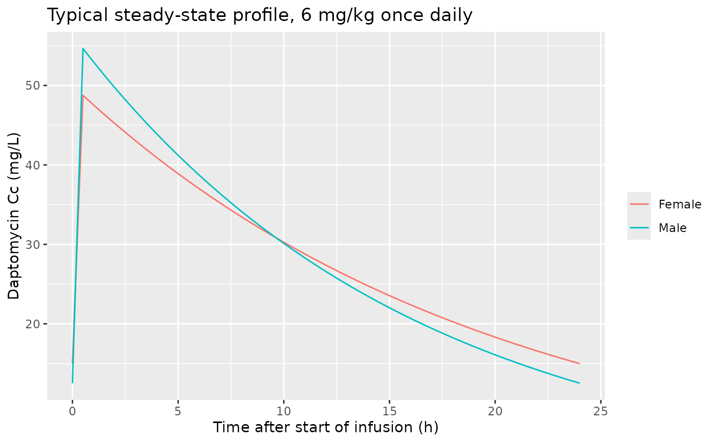
At the Eq 1 reference creatinine clearance (63.35 mL/min), typical CL is 0.636 L/h. Typical V is 10.15 L for men and 12.67 L for women. These give a terminal half-life of about 11-14 h.

mod <- readModelDb("Balice_2022_daptomycin")
mod_typ <- rxode2::zeroRe(mod)
#> ℹ parameter labels from comments will be replaced by 'label()'
#> Warning: No sigma parameters in the model

ev_typ <- tidyr::crossing(
  SEXF = c(0, 1),
  time = c(seq(0, 1, by = 0.05), seq(1.5, 24, by = 0.5))
) |>
  dplyr::mutate(
    id = SEXF + 1L,
    evid = 0L, amt = 0, rate = 0, ii = 0, ss = 0L
  ) |>
  dplyr::bind_rows(
    data.frame(
      id = 1:2, SEXF = c(0, 1), time = 0, evid = 1L,
      amt = 6 * 73, rate = 6 * 73 / 0.5, ii = 24, ss = 1L
    )
  ) |>
  dplyr::mutate(cmt = "central", CRCL = 63.35) |>
  dplyr::arrange(id, time, dplyr::desc(evid))

sim_typ <- rxode2::rxSolve(
  mod_typ, ev_typ,
  maxsteps = 1e6, keep = "SEXF", returnType = "data.frame"
) |>
  dplyr::mutate(sex = ifelse(SEXF == 1, "Female", "Male"))
#> ℹ omega/sigma items treated as zero: 'etacl'
#> Warning: multi-subject simulation without without 'omega'

# Closed form for a one-compartment model at steady state after a 0.5-h
# infusion, sampled after the end of infusion.
closed_ss <- function(dose, cl, v, t, tinf = 0.5, tau = 24) {
  k <- cl / v
  dose / tinf / cl * (1 - exp(-k * tinf)) * exp(-k * (t - tinf)) /
    (1 - exp(-k * tau))
}
chk <- sim_typ |>
  dplyr::filter(time %in% c(1, 23.5)) |>
  dplyr::mutate(
    v = 10.925 + 2.524 * (SEXF - 0.309),
    closed = closed_ss(6 * 73, 0.636, v, time)
  )
knitr::kable(
  chk |>
    dplyr::select(sex, time, Cc, closed) |>
    dplyr::rename(
      "Sex" = sex, "Time after start of infusion (h)" = time,
      "Simulated Cc (mg/L)" = Cc, "Closed form (mg/L)" = closed
    ),
  digits = 2,
  caption = "Typical steady-state peak and trough at 6 mg/kg (438 mg for 73 kg), CRCL 63.35 mL/min."
)

Typical steady-state peak and trough at 6 mg/kg (438 mg for 73 kg), CRCL 63.35 mL/min.
Sex	Time after start of infusion (h)	Simulated Cc (mg/L)	Closed form (mg/L)
Male	1.0	52.95	52.95
Male	23.5	12.92	12.92
Female	1.0	47.55	47.55
Female	23.5	15.37	15.37

# Both sides use the same parameters, so the difference is integration
# error only (LSODA at the default tolerances).
stopifnot(max(abs(chk$Cc / chk$closed - 1)) < 1e-3)

ggplot(sim_typ, aes(time, Cc, colour = sex)) +
  geom_line() +
  labs(
    x = "Time after start of infusion (h)", y = "Daptomycin Cc (mg/L)",
    colour = NULL,
    title = "Typical steady-state profile, 6 mg/kg once daily"
  )

Monte-Carlo probabilities: Table 4 and Figure 5

The paper simulated 10,000 patients from the descriptive statistics of its simulation dataset (n = 134; Table 1: weight 72.9 +/- 10.6 kg, creatinine clearance 74.6 +/- 39.9 mL/min, 44 of 134 female). It reported the probabilities of a trough above the toxicity cut-off of 24.3 mg/L and a peak above the efficacy cut-off of 60 mg/L. Results were given for fixed daily doses (Table 4) and for weight-based dose classes (Figure 5 and Results text). The virtual cohort below uses the same summary statistics, with 200 patients per regimen.

rxode2::rxSetSeed(20220707)
set.seed(20220707)

n_arm <- 200L
make_mc <- function(regimen, dose_mg = NA, dose_mgkg = NA, id_offset) {
  wt <- pmax(rnorm(n_arm, 72.9, 10.6), 40)
  subj <- data.frame(
    id = id_offset + seq_len(n_arm),
    regimen = regimen,
    WT = wt,
    CRCL = pmax(rnorm(n_arm, 74.6, 39.9), 5),
    SEXF = rbinom(n_arm, 1, 44 / 134),
    amt = if (is.na(dose_mg)) dose_mgkg * wt else dose_mg
  )
  dose <- subj |>
    dplyr::mutate(time = 0, evid = 1L, rate = amt / 0.5, ii = 24, ss = 1L)
  obs <- subj |>
    dplyr::select(-amt) |>
    tidyr::crossing(time = c(1, 23.5, 24)) |>
    dplyr::mutate(evid = 0L, amt = 0, rate = 0, ii = 0, ss = 0L)
  dplyr::bind_rows(dose, obs) |>
    dplyr::mutate(cmt = "central") |>
    dplyr::arrange(id, time, dplyr::desc(evid))
}

regimens <- tibble::tribble(
  ~regimen, ~dose_mg, ~dose_mgkg, ~kind,
  "300 mg", 300, NA, "fixed",
  "350 mg", 350, NA, "fixed",
  "400 mg", 400, NA, "fixed",
  "450 mg", 450, NA, "fixed",
  "500 mg", 500, NA, "fixed",
  "550 mg", 550, NA, "fixed",
  "750 mg", 750, NA, "fixed",
  "4-5 mg/kg", NA, 4.5, "weight-based",
  "6-7 mg/kg", NA, 6.5, "weight-based",
  "8-9 mg/kg", NA, 8.5, "weight-based",
  "10-11 mg/kg", NA, 10.5, "weight-based"
)
ev_mc <- dplyr::bind_rows(lapply(seq_len(nrow(regimens)), function(i) {
  make_mc(
    regimens$regimen[i], regimens$dose_mg[i], regimens$dose_mgkg[i],
    id_offset = (i - 1L) * n_arm
  )
}))
stopifnot(!anyDuplicated(unique(ev_mc[, c("id", "time", "evid")])))

sim_mc <- rxode2::rxSolve(
  mod, ev_mc,
  maxsteps = 1e6, keep = "regimen", returnType = "data.frame"
)
#> ℹ parameter labels from comments will be replaced by 'label()'
stopifnot(!anyNA(sim_mc$Cc))

# The paper's probabilities are for model-predicted concentrations: with
# residual error added, the 4-5 mg/kg peak could not stay below 60 mg/L in
# ~99% of patients. The individual prediction Cc is therefore used. Peak = 1 h
# after the start of infusion (the TDM peak time); trough = 24 h (pre-dose).
mc <- sim_mc |>
  dplyr::filter(time %in% c(1, 24)) |>
  dplyr::mutate(what = ifelse(time == 1, "peak", "trough")) |>
  dplyr::select(id, regimen, what, Cc) |>
  tidyr::pivot_wider(names_from = what, values_from = Cc) |>
  dplyr::group_by(regimen) |>
  dplyr::summarise(
    p_cmin = 100 * mean(trough > 24.3),
    p_cmax = 100 * mean(peak > 60),
    .groups = "drop"
  )

# Paper values: Table 4 (fixed doses); Results text for the 6-7 (abstract),
# 8-9 and 10-11 mg/kg classes; 4-5 mg/kg read from Figure 5 by the maintainers.
published_mc <- tibble::tribble(
  ~regimen, ~pub_cmin, ~pub_cmax,
  "300 mg", 2.40, 0.70,
  "350 mg", 6.20, 3.60,
  "400 mg", 8.70, 9.70,
  "450 mg", 10.50, 25.70,
  "500 mg", 16.05, 30.40,
  "550 mg", 21.50, 78.60,
  "750 mg", 44.10, 100,
  "4-5 mg/kg", 5.5, 0.5,
  "6-7 mg/kg", 14.8, 35,
  "8-9 mg/kg", 34.23, 69.24,
  "10-11 mg/kg", 41.58, 81.76
)
mc_cmp <- regimens |>
  dplyr::select(regimen, kind) |>
  dplyr::left_join(published_mc, by = "regimen") |>
  dplyr::left_join(mc, by = "regimen")
stopifnot(nrow(mc_cmp) == 11L, !anyNA(mc_cmp))

mc_cmp |>
  dplyr::rename(
    "Regimen (once daily)" = regimen, "Type" = kind,
    "P(Cmin > 24.3) paper (%)" = pub_cmin,
    "P(Cmin > 24.3) simulated (%)" = p_cmin,
    "P(Cmax > 60) paper (%)" = pub_cmax,
    "P(Cmax > 60) simulated (%)" = p_cmax
  ) |>
  knitr::kable(
    digits = 1,
    caption = "Replicates Table 4 and Figure 5 of Balice 2022 (200 virtual patients per regimen; paper used 10,000)."
  )

Replicates Table 4 and Figure 5 of Balice 2022 (200 virtual patients per regimen; paper used 10,000).
Regimen (once daily)	Type	P(Cmin > 24.3) paper (%)	P(Cmax > 60) paper (%)	P(Cmin > 24.3) simulated (%)	P(Cmax > 60) simulated (%)
300 mg	fixed	2.4	0.7	4.5	1.0
350 mg	fixed	6.2	3.6	8.5	6.0
400 mg	fixed	8.7	9.7	9.0	10.5
450 mg	fixed	10.5	25.7	17.0	21.5
500 mg	fixed	16.0	30.4	16.5	43.0
550 mg	fixed	21.5	78.6	17.5	73.0
750 mg	fixed	44.1	100.0	41.0	100.0
4-5 mg/kg	weight-based	5.5	0.5	6.0	2.5
6-7 mg/kg	weight-based	14.8	35.0	15.0	38.0
8-9 mg/kg	weight-based	34.2	69.2	28.5	80.0
10-11 mg/kg	weight-based	41.6	81.8	43.0	97.0

mc_cmp |>
  tidyr::pivot_longer(
    c(pub_cmin, p_cmin, pub_cmax, p_cmax),
    names_to = "key", values_to = "pct"
  ) |>
  dplyr::mutate(
    source = ifelse(grepl("^pub", key), "Paper", "Simulated"),
    endpoint = ifelse(
      grepl("cmin", key), "P(Cmin > 24.3 mg/L)", "P(Cmax > 60 mg/L)"
    ),
    regimen = factor(regimen, levels = regimens$regimen)
  ) |>
  ggplot(aes(regimen, pct, fill = source)) +
  geom_col(position = "dodge") +
  facet_wrap(~endpoint, ncol = 1) +
  labs(
    x = NULL, y = "Probability (%)", fill = NULL,
    caption = "Replicates Table 4 and Figure 5 of Balice 2022."
  ) +
  theme(axis.text.x = element_text(angle = 45, hjust = 1))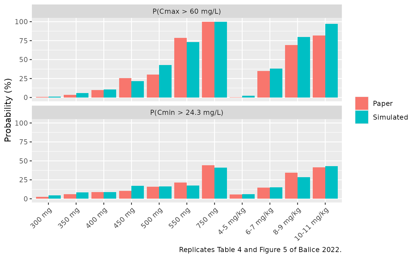

The fixed-dose trough probabilities are the sharpest test of the clearance random effect. Mass-dosed patients differ only through clearance and the sex-dependent volume, so the tail of the trough distribution is set almost entirely by the variance of etacl. The checks below average over the seven fixed doses (1,400 virtual patients). For the trough endpoint, the binomial standard error of that average is about 0.9 percentage points. The model’s long-run value, from a 20,000-patient analytic Monte-Carlo, is 16.2% against the paper’s 15.6%. The two alternative readings of the Table 3 IIV entry discussed under Assumptions give long-run averages of 4.1% and 8.2%. Each is far outside the 5-point bound.

fixed <- dplyr::filter(mc_cmp, kind == "fixed")
stopifnot(
  abs(mean(fixed$p_cmin) - mean(fixed$pub_cmin)) < 5,
  abs(mean(fixed$p_cmax) - mean(fixed$pub_cmax)) < 6
)

Peak and trough concentrations by dose class: Table 2

Table 2 reports the mean measured concentrations 1 h and 23.5 h after the start of infusion, by daily-dose class, across all 155 patients with data. The simulation below uses the full-cohort covariate summary from Table 1 (weight 73.9 +/- 11.2 kg, creatinine clearance 73.6 +/- 38.3 mL/min, 48 of 156 female). It gives each class its midpoint dose and 200 virtual patients. It also samples a dense steady-state grid so that PKNCA can compute exposure. TDM samples are assumed to be at steady state, which the paper does not state.

make_cls <- function(cls, mgkg, id_offset) {
  wt <- pmax(rnorm(n_arm, 73.9, 11.2), 40)
  subj <- data.frame(
    id = id_offset + seq_len(n_arm),
    dose_class = cls,
    CRCL = pmax(rnorm(n_arm, 73.6, 38.3), 5),
    SEXF = rbinom(n_arm, 1, 48 / 156),
    amt = mgkg * wt
  )
  dose <- subj |>
    dplyr::mutate(time = 0, evid = 1L, rate = amt / 0.5, ii = 24, ss = 1L)
  obs <- subj |>
    dplyr::select(-amt) |>
    tidyr::crossing(time = sort(unique(c(seq(0, 1, 0.25), 23.5, seq(2, 24, 1))))) |>
    dplyr::mutate(evid = 0L, amt = 0, rate = 0, ii = 0, ss = 0L)
  dplyr::bind_rows(dose, obs) |>
    dplyr::mutate(cmt = "central") |>
    dplyr::arrange(id, time, dplyr::desc(evid))
}
classes <- tibble::tribble(
  ~dose_class, ~mgkg,
  "4-5 mg/kg", 4.5,
  "6-7 mg/kg", 6.5,
  "8-9 mg/kg", 8.5,
  "10-11 mg/kg", 10.5,
  "12 mg/kg", 12
)
ev_cls <- dplyr::bind_rows(lapply(seq_len(nrow(classes)), function(i) {
  make_cls(classes$dose_class[i], classes$mgkg[i], id_offset = (i - 1L) * n_arm)
}))
stopifnot(!anyDuplicated(unique(ev_cls[, c("id", "time", "evid")])))

sim_cls <- rxode2::rxSolve(
  mod, ev_cls,
  maxsteps = 1e6, keep = "dose_class", returnType = "data.frame"
)
stopifnot(!anyNA(sim_cls$Cc))

# Simulated observations (with residual error, column `sim`) at the TDM
# sampling times, against Table 2 means +/- SD.
tab2 <- tibble::tribble(
  ~dose_class, ~time, ~obs_mean, ~obs_sd,
  "4-5 mg/kg", 1, 45.6, 17.1,
  "6-7 mg/kg", 1, 59.3, 18.0,
  "8-9 mg/kg", 1, 74.4, 51.3,
  "10-11 mg/kg", 1, 69.8, 21.7,
  "12 mg/kg", 1, 80.0, 25.7,
  "4-5 mg/kg", 23.5, 11.4, 8.7,
  "6-7 mg/kg", 23.5, 17.8, 11.0,
  "8-9 mg/kg", 23.5, 15.5, 10.7,
  "10-11 mg/kg", 23.5, 25.4, 14.1,
  "12 mg/kg", 23.5, 17.3, 9.2
)
sim_tdm <- sim_cls |>
  dplyr::filter(time %in% c(1, 23.5)) |>
  dplyr::group_by(dose_class, time) |>
  dplyr::summarise(
    q05 = quantile(sim, 0.05), q50 = median(sim), q95 = quantile(sim, 0.95),
    .groups = "drop"
  ) |>
  dplyr::left_join(tab2, by = c("dose_class", "time")) |>
  dplyr::mutate(dose_class = factor(dose_class, levels = classes$dose_class))

ggplot(sim_tdm, aes(dose_class)) +
  geom_linerange(aes(ymin = q05, ymax = q95), colour = "steelblue", linewidth = 4, alpha = 0.4) +
  geom_point(aes(y = q50), colour = "steelblue", size = 2) +
  geom_pointrange(
    aes(y = obs_mean, ymin = obs_mean - obs_sd, ymax = obs_mean + obs_sd),
    colour = "firebrick", position = position_nudge(x = 0.2)
  ) +
  facet_wrap(~ paste0(time, " h after start of infusion"), scales = "free_y") +
  labs(
    x = "Daily dose class", y = "Daptomycin (mg/L)",
    caption = paste(
      "Blue: simulated median and 5th-95th percentiles with residual error.",
      "Red: Table 2 observed mean +/- SD (Balice 2022)."
    )
  ) +
  theme(axis.text.x = element_text(angle = 45, hjust = 1))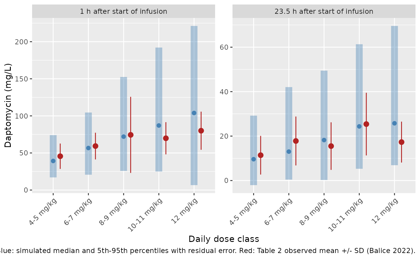

PKNCA validation

PKNCA computes the steady-state exposure for each dose class. A 1-23.5 h interval reproduces the TDM sampling design: its cmax is the 1-h peak and its cmin the 23.5-h trough. A 0-24 h interval gives the dosing-interval AUC. Table 2 reports arithmetic means, so the simulated values are summarised as per-class means before comparison.

sim_nca <- sim_cls |>
  dplyr::filter(!is.na(Cc)) |>
  dplyr::select(id, time, Cc, dose_class)
# The observation grid carries a time-zero (steady-state pre-dose) row for
# every subject, so the 0-24 h AUC is anchored without adding rows.
stopifnot(
  all(tapply(sim_nca$time == 0, sim_nca$id, any)),
  !anyNA(sim_nca$Cc)
)

conc_obj <- PKNCA::PKNCAconc(sim_nca, Cc ~ time | dose_class + id)
dose_df <- ev_cls |>
  dplyr::filter(evid == 1) |>
  dplyr::select(id, time, amt, dose_class)
dose_obj <- PKNCA::PKNCAdose(dose_df, amt ~ time | dose_class + id)

intervals <- data.frame(
  start = c(1, 0), end = c(23.5, 24),
  cmax = c(TRUE, FALSE), cmin = c(TRUE, FALSE),
  auclast = c(FALSE, TRUE)
)
nca_res <- PKNCA::pk.nca(PKNCA::PKNCAdata(conc_obj, dose_obj, intervals = intervals))

nca_ind <- as.data.frame(nca_res) |>
  dplyr::filter(PPTESTCD %in% c("cmax", "cmin", "auclast")) |>
  dplyr::select(id, dose_class, PPTESTCD, PPORRES) |>
  tidyr::pivot_wider(names_from = PPTESTCD, values_from = PPORRES)

# AUC over the steady-state dosing interval must equal dose / CL (paper
# Methods 4.5: 'AUC = dose/Cl'); the residual is trapezoid error on the
# hourly grid.
auc_chk <- nca_ind |>
  dplyr::left_join(dose_df |> dplyr::select(id, amt), by = "id") |>
  dplyr::left_join(
    sim_cls |> dplyr::distinct(id, cl),
    by = "id"
  ) |>
  dplyr::mutate(ratio = auclast / (amt / cl))
stopifnot(abs(median(auc_chk$ratio) - 1) < 0.02)

sim_means <- nca_ind |>
  dplyr::group_by(dose_class) |>
  dplyr::summarise(
    cmax = mean(cmax), cmin = mean(cmin), auclast = mean(auclast),
    .groups = "drop"
  )
reference <- tab2 |>
  dplyr::mutate(code = ifelse(time == 1, "cmax", "cmin")) |>
  dplyr::select(dose_class, code, obs_mean) |>
  tidyr::pivot_wider(names_from = code, values_from = obs_mean)

cmp <- nlmixr2lib::ncaComparisonTable(
  simulated = sim_means,
  reference = reference,
  by = "dose_class",
  params = c("cmax", "cmin"),
  units = c(cmax = "mg/L", cmin = "mg/L"),
  tolerance_pct = 20
)
knitr::kable(
  cmp,
  caption = paste(
    "Simulated steady-state mean 1-h peak (Cmax) and 23.5-h trough (Cmin)",
    "versus Table 2 observed means. * differs from reference by >20%."
  )
)

Simulated steady-state mean 1-h peak (Cmax) and 23.5-h trough (Cmin) versus Table 2 observed means. * differs from reference by >20%.
NCA parameter	dose_class	Reference	Simulated	% diff
Cmax (mg/L)	4-5 mg/kg	45.6	40.4	-11.3%
Cmax (mg/L)	6-7 mg/kg	59.3	58	-2.2%
Cmax (mg/L)	8-9 mg/kg	74.4	74.1	-0.4%
Cmax (mg/L)	10-11 mg/kg	69.8	92.8	+32.9%*
Cmax (mg/L)	12 mg/kg	80	109	+36.2%*
Cmin (mg/L)	4-5 mg/kg	11.4	11.7	+2.6%
Cmin (mg/L)	6-7 mg/kg	17.8	16.7	-6.0%
Cmin (mg/L)	8-9 mg/kg	15.5	20.9	+34.8%*
Cmin (mg/L)	10-11 mg/kg	25.4	26.9	+6.0%
Cmin (mg/L)	12 mg/kg	17.3	32.2	+86.1%*


sim_means |>
  dplyr::mutate(dose_class = factor(dose_class, levels = classes$dose_class)) |>
  dplyr::arrange(dose_class) |>
  dplyr::rename(
    "Dose class" = dose_class, "Mean 1-h peak (mg/L)" = cmax,
    "Mean 23.5-h trough (mg/L)" = cmin, "Mean AUC0-24,ss (mg*h/L)" = auclast
  ) |>
  knitr::kable(digits = 1, caption = "Simulated steady-state exposure by dose class.")

Simulated steady-state exposure by dose class.
Dose class	Mean 1-h peak (mg/L)	Mean 23.5-h trough (mg/L)	Mean AUC0-24,ss (mg*h/L)
4-5 mg/kg	40.4	11.7	554.7
6-7 mg/kg	58.0	16.7	794.4
8-9 mg/kg	74.1	20.9	1007.0
10-11 mg/kg	92.8	26.9	1275.1
12 mg/kg	108.9	32.2	1508.5


# The 6-7 mg/kg class holds 96 of the 155 patients, so its observed means are
# the most precise (SE of the mean about 1.8 mg/L for the peak and 1.1 mg/L
# for the trough).
ref67 <- dplyr::filter(sim_means, dose_class == "6-7 mg/kg")
stopifnot(
  abs(ref67$cmax / 59.3 - 1) < 0.15,
  abs(ref67$cmin / 17.8 - 1) < 0.25
)

The 6-7 mg/kg class holds 96 of the 155 patients. There, the simulated mean peak and trough agree with the observed means. The flagged rows are in the sparse classes. The observed means there do not rise with dose: the 12 mg/kg trough (17.3 mg/L) is below the 10-11 mg/kg trough (25.4 mg/L), and the 8-9 mg/kg trough is below the 6-7 mg/kg trough. The model’s prediction rises with dose, as a linear model must. The paper itself notes that the 10 mg/kg peak “seems lower than expected” and the trough higher. It attributes this to the 10-12 mg/kg regimens being the least often prescribed (8 and 4 patients), which makes those means “more susceptible to random sampling fluctuation”. Dose adjustments made in response to TDM may also contribute; this is not stated in the paper. Doses within each class also vary around the simulated midpoint.

Assumptions and deviations

Additive random effect on clearance, entered as a variance. Eq 1 prints + eta on the linear CL scale, so etacl is additive in L/h. The Table 3 entry “IIV Cl = 0.027” is taken as the NONMEM OMEGA variance, giving an SD of 0.164 L/h, about 25% of the typical CL. The abstract and Discussion describe this as “2.7% IIV”, which restates the variance as a percentage. The maintainers tested three readings against the paper’s Monte-Carlo Table 4. Only the variance reading reproduces it: the fixed-dose trough probabilities average 16.2% (model, analytic 20,000-patient Monte-Carlo) against the paper’s 15.6%. Reading 0.027 as an additive SD gives 4.1%, and reading it as a log-normal variance gives 8.2%. An additive normal effect can in principle make CL negative. With the published values that needs an eta about 4 SD below zero (probability about 4e-5 per subject), and no such subject arises at the cohort sizes used here.
Residual error form. The paper describes the residual model only in words: an intercept-plus-slope model in the additive and proportional thetas below an IPRED of 80 mg/L, and a model “proportional to a lone third parameter” above it. It is encoded as SD = theta3 + theta4 x IPRED below 80 mg/L and SD = |theta7| x IPRED at or above. The negative sign of theta7 is immaterial because NONMEM uses the SD squared. A continuous form (theta7 as a change in slope above 80 mg/L) and a quadrature-summed form below 80 mg/L were also simulated. Only the forms with the theta7-proportional branch reproduce the wide upper 95th-percentile band (about 100-178 mg/L) of the Figure 3 VPC at the 1-h peak. The residual SD is discontinuous at 80 mg/L (27.5 vs 43.7 mg/L), as the verbal description implies.
Creatinine clearance units. Table 1 labels creatinine clearance mL/min/1.73 m^2, but Methods 4.1 states it was calculated with the Cockcroft-Gault equation, which yields raw mL/min. The model follows the Methods; supply raw Cockcroft-Gault mL/min. Because the CL slope is only 0.109 L/h per 100 mL/min, the choice changes CL by a few percent at most.
Centring constants. 63.35 mL/min (Eq 1) is not identified in the paper as a cohort statistic. 0.309 (Eq 2) equals the female fraction of the model-building subset (29/94).
Sex effect direction. With theta6 = -2.524 entering as - theta6 x (Sex - 0.309), women have the larger volume (12.67 vs 10.15 L), as printed. The paper does not state the direction in words.
Monte-Carlo cohort. Weight and creatinine clearance were drawn from normal distributions with the Table 1 means and SDs, truncated at 40 kg and 5 mL/min. The paper does not state its sampling distributions or truncation. Weight-based dose classes were simulated at their midpoints. The 4-5 mg/kg probabilities and the 6-7 mg/kg peak probability were read from Figure 5 by the maintainers; the other values are printed. The peak was taken 1 h after the start of infusion and the trough at 24 h, both at steady state. The probabilities use model-predicted concentrations, without residual error.
Steady state for the TDM comparison. Table 2 samples are compared with steady-state simulations. The paper does not report on which day TDM samples were drawn.
Not reproduced. The supplementary probability-of-target-attainment tables (S1-S3) and Figure 6 depend on EUCAST MIC distributions that are not reproduced here.
No correction notice for this article was found in Europe PMC as of 2026-10-03.