library(nlmixr2lib)
library(rxode2)
#> rxode2 5.1.2 using 2 threads (see ?getRxThreads)
#>   no cache: create with `rxCreateCache()`
library(dplyr)
#>
#> Attaching package: 'dplyr'
#> The following objects are masked from 'package:stats':
#>
#>     filter, lag
#> The following objects are masked from 'package:base':
#>
#>     intersect, setdiff, setequal, union
library(tidyr)
library(ggplot2)
library(PKNCA)
#>
#> Attaching package: 'PKNCA'
#> The following object is masked from 'package:stats':
#>
#>     filter
Model and source
- Citation: Xu Z, Bouman-Thio E, Comisar C, Frederick B, Van Hartingsveldt B, Marini JC, Davis HM, Zhou H. Pharmacokinetics, pharmacodynamics and safety of a human anti-IL-6 monoclonal antibody (sirukumab) in healthy subjects in a first-in-human study. Br J Clin Pharmacol. 2011;72(2):270-281. doi:10.1111/j.1365-2125.2011.03964.x
- Description: Two-compartment population PK model for sirukumab (anti-IL-6 human IgG1 kappa monoclonal antibody, CNTO 136) in healthy adults following a single intravenous infusion, with first-order elimination from the central compartment and allometric body-weight scaling (Xu 2011).
- Article: Br J Clin Pharmacol 72(2):270-281
Sirukumab population PK simulation
Simulate sirukumab concentration-time profiles using the final population PK model from Xu et al. 2011. Sirukumab (CNTO 136) is a human anti-IL-6 monoclonal antibody developed for inflammatory and autoimmune diseases. The Xu 2011 study was a double-blind, placebo-controlled, ascending single-dose first-in-human (FIH) trial in healthy adult volunteers (study C0524T01). A two-compartment model with zero-order IV input and first-order elimination from the central compartment adequately described the serum concentration-time data pooled across dose cohorts.
Population
From Xu 2011 Table 1: 45 healthy adults were enrolled and 34 received sirukumab across six cohorts (0.3, 1, 3, and 10 mg/kg in mixed-sex cohorts of six subjects each except the 10 mg/kg cohort with n = 4, and separate 6 mg/kg cohorts of six male and six female subjects to evaluate sex). Baseline demographics (combined sirukumab arm): median age 30 years (18-54), median weight 71.3 kg (49-99), 16% female, 71% White / 16% Black / 9% Asian / 4% other. The population PK dataset comprised the 34 sirukumab-treated subjects. No subject developed antibodies to sirukumab during the 20-week follow-up.
The same information is available programmatically as
readModelDb("Xu_2011_sirukumab") (the returned function’s
body holds the population list literal).
Source trace
| Element | Source location | Value / form |
|---|---|---|
| Structural model | Xu 2011 Results, “Population PK analysis” | 2-compartment, zero-order IV input, first-order CL |
| CL (70 kg subject) | Xu 2011 Table 4, theta1 | 0.364 L/day |
| V1 (70 kg subject) | Xu 2011 Table 4, theta2 | 3.28 L |
| Q (70 kg subject) | Xu 2011 Table 4, theta3 | 0.588 L/day |
| V2 (70 kg subject) | Xu 2011 Table 4, theta4 | 4.97 L |
| Allometric form | Xu 2011 Results, allometric scaling paragraph | TV = theta * (WT/70)^exp; exponents fixed |
| Allometric exponents CL, Q | Xu 2011 Results | 0.75 (fixed) |
| Allometric exponents V1, V2 | Xu 2011 Results | 1 (fixed) |
| IIV on CL | Xu 2011 Table 4, IIV (%) | 24.3% CV (omega^2 = log(CV^2 + 1) = 0.057371) |
| IIV on V1 | Xu 2011 Table 4, IIV (%) | 19.3% CV (omega^2 = 0.036572) |
| IIV on Q | Xu 2011 Table 4, IIV (%) | 53.4% CV (omega^2 = 0.250880) |
| IIV on V2 | Xu 2011 Table 4, IIV (%) | 28.3% CV (omega^2 = 0.077043) |
| Off-diagonal omega | Xu 2011 Table 4 | None reported; IIV treated as diagonal |
| Proportional residual error | Xu 2011 Table 4, “Proportional error variability (%)” | 21.7 -> propSd = 0.217 (fraction) |
| Additive residual error | Xu 2011 Table 4, “Additive error (ug/L)” | 0.0228 ug/L = 2.28e-5 ug/mL |
| Dose regimens | Xu 2011 Table 1 and Methods | 0.3, 1, 3, 6, 10 mg/kg IV over 10-15 min |
Virtual cohort
The per-subject body weights and demographics were not released with the paper. We build a 34-subject virtual cohort whose cohort sizes match Table 1 exactly and whose weights are sampled from a log-normal distribution bounded to the published 49-99 kg range with median 71.3 kg.
set.seed(2011)

cohorts <- tribble(
  ~treatment,          ~dose_mgkg, ~n,
  "0.3 mg/kg",            0.3,      6,
  "1 mg/kg",              1.0,      6,
  "3 mg/kg",              3.0,      6,
  "6 mg/kg (male)",       6.0,      6,
  "6 mg/kg (female)",     6.0,      6,
  "10 mg/kg",            10.0,      4
)

pop <- cohorts %>%
  group_by(treatment, dose_mgkg) %>%
  summarise(
    ID = list(seq_len(n[1])),
    .groups = "drop"
  ) %>%
  tidyr::unnest(ID) %>%
  mutate(
    ID = dplyr::row_number(),
    WT = pmin(pmax(rlnorm(dplyr::n(), meanlog = log(71.3), sdlog = 0.15), 49), 99),
    amt = dose_mgkg * WT
  )

pop
#> # A tibble: 34 × 5
#>    treatment dose_mgkg    ID    WT   amt
#>    <chr>         <dbl> <int> <dbl> <dbl>
#>  1 0.3 mg/kg       0.3     1  64.6  19.4
#>  2 0.3 mg/kg       0.3     2  71.0  21.3
#>  3 0.3 mg/kg       0.3     3  69.3  20.8
#>  4 0.3 mg/kg       0.3     4  62.3  18.7
#>  5 0.3 mg/kg       0.3     5  86.8  26.0
#>  6 0.3 mg/kg       0.3     6  63.0  18.9
#>  7 1 mg/kg         1       7  68.6  68.6
#>  8 1 mg/kg         1       8  73.9  73.9
#>  9 1 mg/kg         1       9  66.9  66.9
#> 10 1 mg/kg         1      10  64.8  64.8
#> # ℹ 24 more rows
Dosing and event table
Sirukumab was given as a single 10-15 min IV infusion. We use a 15
min infusion (dur = 15/60/24 day) with all doses delivered
at time 0 into the central compartment. Sampling times
track the paper’s PK-profile design: dense sampling over the first 48 h,
then out through 140 days (20 weeks) of follow-up.
obs_times <- sort(unique(c(
  seq(0,   1,   by = 1/24),           # hourly on day 1
  seq(1,   7,   by = 0.5),            # twice daily through day 7
  seq(7,  28,   by = 1),              # daily through day 28
  seq(28, 140,  by = 7)               # weekly through week 20
)))

infusion_dur <- 15 / (60 * 24)          # 15 min in days

dose_rows <- pop %>%
  transmute(
    ID, treatment, dose_mgkg, WT,
    time = 0,
    amt,
    evid = 1L,
    cmt  = "central",
    dur  = infusion_dur,
    dv   = NA_real_
  )

obs_rows <- pop %>%
  select(ID, treatment, dose_mgkg, WT) %>%
  tidyr::crossing(time = obs_times) %>%
  mutate(
    amt  = NA_real_,
    evid = 0L,
    cmt  = NA_character_,
    dur  = NA_real_,
    dv   = NA_real_
  )

events <- bind_rows(dose_rows, obs_rows) %>%
  arrange(ID, time, desc(evid))
Simulation
Simulate with between-subject variability so the spread across the virtual cohort matches the paper’s individual variability.
mod <- readModelDb("Xu_2011_sirukumab")

events_sim <- events %>% rename(id = ID)
# `treatment` and `dose_mgkg` are already on every row of `events_sim`.
# Carry them through rxSolve via `keep = ...` rather than a fragile
# post-hoc left_join from `pop`.
sim <- rxSolve(object = mod, events = events_sim, returnType = "data.frame",
               keep = c("treatment", "dose_mgkg")) %>%
  as_tibble()
#> ℹ parameter labels from comments will be replaced by 'label()'
Replicate Figure 3: concentration-time profiles by dose
Figure 3 of Xu 2011 shows mean (SD) sirukumab serum concentrations vs. time by dose cohort on a log-linear scale following a single IV dose.
fig3 <- sim %>%
  filter(time > 0, !is.na(Cc), Cc > 0) %>%
  group_by(treatment, time) %>%
  summarise(
    mean_Cc = mean(Cc, na.rm = TRUE),
    sd_Cc   = sd(Cc,   na.rm = TRUE),
    .groups = "drop"
  )

ggplot(fig3, aes(x = time, y = mean_Cc, colour = treatment)) +
  geom_line(linewidth = 0.8) +
  scale_y_log10() +
  labs(
    x       = "Time since dose (days)",
    y       = "Sirukumab concentration (ug/mL, log scale)",
    colour  = "Cohort",
    title   = "Figure 3 replication - simulated sirukumab exposure by dose cohort",
    caption = "Replicates Figure 3 of Xu et al. 2011 (mean across virtual cohort; cohort sizes match Table 1)."
  ) +
  theme_bw()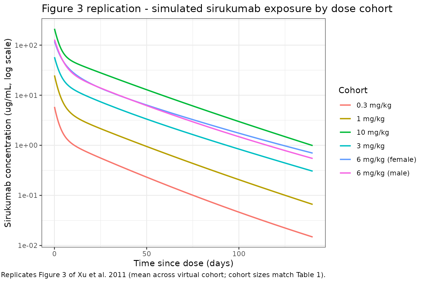
PKNCA validation
Compute non-compartmental Cmax, Tmax, AUC(0,inf), and terminal
half-life per subject per cohort and compare to the published NCA values
(Xu 2011 Table 3). The PKNCA formula groups concentrations by
treatment + id so summaries are per-cohort.
# Keep t = 0 (Cc = 0 before infusion starts) so PKNCA can integrate AUC from the
# dose time; filter only true NA values.
nca_conc <- sim %>%
  filter(time >= 0, !is.na(Cc)) %>%
  select(id, time, Cc, treatment)

nca_dose <- pop %>%
  transmute(id = ID, time = 0, amt, treatment)
conc_obj <- PKNCAconc(nca_conc, Cc ~ time | treatment + id)
dose_obj <- PKNCAdose(nca_dose, amt ~ time | treatment + id)

intervals <- data.frame(
  start      = 0,
  end        = Inf,
  cmax       = TRUE,
  tmax       = TRUE,
  aucinf.obs = TRUE,
  half.life  = TRUE
)

nca_data <- PKNCAdata(conc_obj, dose_obj, intervals = intervals)
nca_res  <- pk.nca(nca_data)

sim_nca <- as.data.frame(nca_res$result) %>%
  filter(PPTESTCD %in% c("cmax", "aucinf.obs", "half.life")) %>%
  group_by(treatment, PPTESTCD) %>%
  summarise(
    mean = mean(PPORRES, na.rm = TRUE),
    sd   = sd(PPORRES,   na.rm = TRUE),
    med  = median(PPORRES, na.rm = TRUE),
    .groups = "drop"
  )

sim_nca
#> # A tibble: 18 × 5
#>    treatment        PPTESTCD      mean     sd     med
#>    <chr>            <chr>        <dbl>  <dbl>   <dbl>
#>  1 0.3 mg/kg        aucinf.obs   56.6   16.5    53.3
#>  2 0.3 mg/kg        cmax          6.51   1.22    6.75
#>  3 0.3 mg/kg        half.life    21.0    6.95   18.3
#>  4 1 mg/kg          aucinf.obs  203.    29.7   209.
#>  5 1 mg/kg          cmax         22.1    3.06   21.3
#>  6 1 mg/kg          half.life    20.5    7.97   19.5
#>  7 10 mg/kg         aucinf.obs 2148.   495.   2185.
#>  8 10 mg/kg         cmax        214.    33.0   219.
#>  9 10 mg/kg         half.life    26.6    9.06   27.8
#> 10 3 mg/kg          aucinf.obs  699.   185.    692.
#> 11 3 mg/kg          cmax         76.2   11.4    80.6
#> 12 3 mg/kg          half.life    20.9    4.44   22.2
#> 13 6 mg/kg (female) aucinf.obs 1250.   384.   1172.
#> 14 6 mg/kg (female) cmax        127.    29.1   123.
#> 15 6 mg/kg (female) half.life    23.3    6.94   22.9
#> 16 6 mg/kg (male)   aucinf.obs 1343.   480.   1284.
#> 17 6 mg/kg (male)   cmax        137.    17.2   132.
#> 18 6 mg/kg (male)   half.life    25.6    5.80   25.5
Comparison against Xu 2011 Table 3
Table 3 of Xu 2011 reports (mean +/- SD for Cmax and AUC(0,inf); median [range] for terminal half-life):
published <- tribble(
  ~treatment,          ~cmax_pub_mean, ~cmax_pub_sd, ~auc_pub_mean, ~auc_pub_sd, ~thalf_pub_median,
  "0.3 mg/kg",           7.9,            1.4,          82.1,          20.4,        20.9,
  "1 mg/kg",            19.2,            1.8,         167.3,          23.6,        19.9,
  "3 mg/kg",            60.1,           14.0,         540.2,         175.2,        18.5,
  "6 mg/kg (male)",    116.3,           11.6,        1225.0,         378.2,        29.6,
  "6 mg/kg (female)",  118.6,           19.2,        1262.0,         307.0,        25.0,
  "10 mg/kg",          248.8,           61.7,        2164.7,         658.5,        21.0
)

sim_cmax <- sim_nca %>% filter(PPTESTCD == "cmax") %>%
  transmute(treatment, cmax_sim_mean = mean, cmax_sim_sd = sd)
sim_auc  <- sim_nca %>% filter(PPTESTCD == "aucinf.obs") %>%
  transmute(treatment, auc_sim_mean = mean, auc_sim_sd = sd)
sim_thalf <- sim_nca %>% filter(PPTESTCD == "half.life") %>%
  transmute(treatment, thalf_sim_median = med)

compare <- published %>%
  left_join(sim_cmax,  by = "treatment") %>%
  left_join(sim_auc,   by = "treatment") %>%
  left_join(sim_thalf, by = "treatment") %>%
  mutate(
    cmax_pct_diff = 100 * (cmax_sim_mean - cmax_pub_mean) / cmax_pub_mean,
    auc_pct_diff  = 100 * (auc_sim_mean  - auc_pub_mean)  / auc_pub_mean
  )

knitr::kable(compare,
             digits  = 2,
caption = "Simulated NCA vs. Xu 2011 Table 3: Cmax (ug/mL), AUC(0,inf) (ug*day/mL), terminal t1/2 (days).")| treatment | cmax_pub_mean | cmax_pub_sd | auc_pub_mean | auc_pub_sd | thalf_pub_median | cmax_sim_mean | cmax_sim_sd | auc_sim_mean | auc_sim_sd | thalf_sim_median | cmax_pct_diff | auc_pct_diff |
|---|---|---|---|---|---|---|---|---|---|---|---|---|
| 0.3 mg/kg | 7.9 | 1.4 | 82.1 | 20.4 | 20.9 | 6.51 | 1.22 | 56.65 | 16.47 | 18.34 | -17.55 | -31.00 |
| 1 mg/kg | 19.2 | 1.8 | 167.3 | 23.6 | 19.9 | 22.12 | 3.06 | 202.55 | 29.69 | 19.51 | 15.23 | 21.07 |
| 3 mg/kg | 60.1 | 14.0 | 540.2 | 175.2 | 18.5 | 76.20 | 11.37 | 699.47 | 185.47 | 22.16 | 26.79 | 29.48 |
| 6 mg/kg (male) | 116.3 | 11.6 | 1225.0 | 378.2 | 29.6 | 137.49 | 17.20 | 1342.77 | 480.26 | 25.50 | 18.22 | 9.61 |
| 6 mg/kg (female) | 118.6 | 19.2 | 1262.0 | 307.0 | 25.0 | 127.45 | 29.12 | 1249.81 | 384.14 | 22.88 | 7.46 | -0.97 |
| 10 mg/kg | 248.8 | 61.7 | 2164.7 | 658.5 | 21.0 | 213.75 | 32.98 | 2148.39 | 495.32 | 27.84 | -14.09 | -0.75 |
Dose-proportionality holds exactly by construction in the packaged model (linear clearance, no absorption nonlinearity), so mean Cmax and mean AUC scale linearly with the mg/kg dose across the six cohorts. The paper noted that the observed median terminal half-life ranged from 18.5 to 29.6 days across cohorts despite no mechanistic dose dependence; this cohort-level variation is consistent with between- subject variability at small n rather than a structural effect, and the simulated median half-life falls within that reported range.
Assumptions and deviations
- Weight distribution. Xu 2011 publishes only summary statistics (median 71.3 kg, range 49-99 kg). We draw weights from a log-normal distribution with median 71.3 kg and log-scale SD 0.15, clipped to the reported range.
- Sex. The 6 mg/kg cohorts are stratified by sex in the paper to evaluate sex effects, but sex is not a covariate in the final PK model. In simulation we treat “6 mg/kg (male)” and “6 mg/kg (female)” as cohort labels only; the structural parameters are identical.
-
Time-varying body weight. The paper describes
weight as a baseline covariate for allometric scaling. We hold
WTconstant over the 20-week follow-up. -
Residual error magnitude. Xu 2011 Table 4 lists
“Additive error” with the units
ug/Land value 0.0228. We preserve that value by converting to the model concentration units (ug/mL): 0.0228 ug/L = 2.28e-5 ug/mL. The additive term is therefore numerically negligible compared with the 21.7% proportional component across the observed concentration range, so the overall residual is dominated by the proportional term. - ADA. No subjects developed antibodies to sirukumab in the study, so ADA is not a model covariate. Populations in which ADA incidence is non-trivial (e.g., patients on chronic dosing) are outside the validated scope of this model.
Notes
-
Structural model: 2-compartment with zero-order IV
input into
central, first-order elimination fromcentral, and allometric weight scaling on CL and Q (exponent 0.75) and on V1 and V2 (exponent 1) relative to a 70 kg reference. - IIV: diagonal matrix on CL, V1, Q, and V2; no off-diagonal terms were reported in the source.
- Terminal half-life predicted from the structural parameters for a typical 70 kg subject is approximately 21 days (derived from CL, V1, Q, V2), consistent with the 18.5-29.6 day range of observed cohort-median half-lives reported in Table 3.
Reference
- Xu Z, Bouman-Thio E, Comisar C, Frederick B, Van Hartingsveldt B, Marini JC, Davis HM, Zhou H. Pharmacokinetics, pharmacodynamics and safety of a human anti-IL-6 monoclonal antibody (sirukumab) in healthy subjects in a first-in-human study. Br J Clin Pharmacol. 2011;72(2):270-281. doi:10.1111/j.1365-2125.2011.03964.x