Palbociclib PK and myelosuppression in children (Panetta 2024)
Source:vignettes/articles/Panetta_2024_palbociclib.Rmd
Panetta_2024_palbociclib.RmdModel and source
Panetta et al. (2024) reported the first population pharmacokinetic and pharmacodynamic analysis of palbociclib in children, using the Pediatric Brain Tumor Consortium phase 1 study PBTC-042 (NCT02255461). Three models were fitted and each has its own parameter table, so each is packaged as its own model file:
| Model file | Paper’s model | Parameter source | Output |
|---|---|---|---|
Panetta_2024_palbociclib |
Population PK, final (AST) model | Table 2, AST column | Palbociclib plasma concentration |
Panetta_2024_palbociclib_anc |
Neutrophil PD model | Table 3A (+ Table 2 PK) | ANC |
Panetta_2024_palbociclib_plt |
Platelet PD model | Table 3B (+ Table 2 PK) | Platelet count |
The two pharmacodynamic models were estimated separately, with the palbociclib pharmacokinetics fixed to each individual’s post hoc estimates (section 2.4.2), so they share no parameters with each other. Section 2.4.1 states only that “we used a similar structural model for platelet dynamics” – the structure is common, the numbers are not.
- Article: https://doi.org/10.3390/pharmaceutics16121528
- Supplementary material: https://www.mdpi.com/article/10.3390/pharmaceutics16121528/s1
mod_pk  <- rxode2::rxode(readModelDb("Panetta_2024_palbociclib"))
#> ℹ parameter labels from comments will be replaced by 'label()'
#> Warning: some etas defaulted to non-mu referenced, possible parsing error: etaiov_cl_1, etaiov_cl_2
#> as a work-around try putting the mu-referenced expression on a simple line
mod_anc <- rxode2::rxode(readModelDb("Panetta_2024_palbociclib_anc"))
#> ℹ parameter labels from comments will be replaced by 'label()'
#> Warning: some etas defaulted to non-mu referenced, possible parsing error: etaiov_kin_1, etaiov_kin_2, etaiov_ic50_1, etaiov_ic50_2, etaiov_fktr_1, etaiov_fktr_2, etaiov_cl_1, etaiov_cl_2
#> as a work-around try putting the mu-referenced expression on a simple line
mod_plt <- rxode2::rxode(readModelDb("Panetta_2024_palbociclib_plt"))
#> ℹ parameter labels from comments will be replaced by 'label()'
#> Warning: some etas defaulted to non-mu referenced, possible parsing error: etaiov_kin_1, etaiov_kin_2, etaiov_ic50_1, etaiov_ic50_2, etaiov_fktr_1, etaiov_fktr_2, etaiov_cl_1, etaiov_cl_2
#> as a work-around try putting the mu-referenced expression on a simple line- Citation: Panetta JC, Selvo NS, Van Mater D, Stewart CF. (2024). Population Pharmacokinetic and Pharmacodynamic Study of Palbociclib in Children and Young Adults with Recurrent, Progressive, or Refractory Brain Tumors. Pharmaceutics 16(12):1528. doi:10.3390/pharmaceutics16121528. The underlying phase 1 trial is PBTC-042 (NCT02255461).
The PK model runs in hours, matching Table 2. Both PD models run in
days, matching Table 3, and carry the PK layer with its rate constants
converted inline (log(0.46 * 24),
log(36.5 * 24), log(0.8 / 24)).
Units and BSA
Panetta 2024 reports V/F in L/m^2 and CL/F
in L/h/m^2, and section 2.3 states that “the palbociclib dosage (i.e.,
the palbociclib dosage normalized to the patient body surface area
(BSA)) was used as the model input”. Doses are therefore supplied in
mg/m^2, body-surface area cancels out of the model
entirely, and no BSA covariate is required. central / vc is
in mg/L, so the observation equation multiplies by 1000 to give the
ng/mL that the paper plots. A clinical dose in mg becomes
amt = dose / BSA.
Population
Thirty-four patients aged 4.9-21.6 years (median 12.8) with recurrent, progressive or refractory brain tumors were enrolled; one was excluded for taking phenytoin and omeprazole against protocol, leaving 33 in the PK analysis and 387 evaluable concentrations. Median weight was 52.5 kg (23.8-110.4) and median BSA 1.5 m^2 (0.8-2.4); 36% were female and 58% Caucasian. Patients were split into stratum I (21 patients, not heavily pretreated) and stratum II (12 patients, heavily pretreated). Oral palbociclib was given at 50 (6 patients), 75 (21) or 95 mg/m^2 (6) once daily for 21 days of each 28-day course. Baseline laboratory medians (range) were albumin 4.2 g/dL (3.2-4.9), AST 25 U/L (11-93), bilirubin 0.4 mg/dL (0.1-1.2) and creatinine 0.5 mg/dL (0.2-1.2) (Table 1).
Two of the 33 patients had only a single pre-treatment blood count and were excluded from the pharmacodynamic analysis, which used 190 ANC and 189 platelet observations from 31 patients in course 1 and 99 of each in course 2.
The same information is available programmatically via each model’s
population metadata, e.g.
readModelDb("Panetta_2024_palbociclib")()$population.
Source trace
The per-parameter origin is recorded as an in-file comment next to
each ini() entry in
inst/modeldb/specificDrugs/Panetta_2024_palbociclib*.R. The
table below collects them in one place.
| Equation / parameter | Value | Source location |
|---|---|---|
ltlag (Tlag) |
0.8 h | Table 2, AST column |
lka (ka) |
0.46 /h | Table 2, AST column |
lvc (V/F) |
653 L/m^2 | Table 2, AST column |
lcl (CL/F) |
36.5 L/h/m^2 | Table 2, AST column |
e_ast_cl |
-0.3 | Table 2, AST column; p = 0.0066 |
| AST centring value | 25 U/L | Table 1 (cohort median); section 2.3.1 |
etaltlag, etalka, etalvc,
etalcl
|
0.67, 0.87, 0.04, 0.26 (SD) | Table 2, AST column; footnote “IIV and IOV are reported as a standard deviation” |
etaiov_cl_1/2 |
0.12 (SD) | Table 2, AST column |
propSd |
0.32 | Table 2, AST column |
ANC lrbase (Ncirc0) |
3.95 x 10^3/uL | Table 3A |
ANC lkin, logitfktr,
lic50
|
0.90 /day, 0.78/0.90, 383.5 | Table 3A |
ANC lkout, lhill
|
4.80 /day, 1 (both fixed) | Table 3A |
| ANC IIV / IOV | CV% per Table 3A | Table 3A |
ANC propSd_ANC
|
0.29 | Table 3A (b) |
PLT lrbase (Ncirc0) |
267.40 x 10^9/L | Table 3B |
PLT lkin, logitfktr,
lic50
|
0.93 /day, 0.52/0.93, 559.14 | Table 3B |
PLT lkout, lhill
|
4.80 /day, 1 (both fixed) | Table 3B |
PLT propSd_PLT
|
0.20 | Table 3B (b) |
| One-compartment PK with lag | n/a | Section 2.3 |
| Marrow / transit / circulating ODEs | n/a | Equations 1-5 and Figure S1 |
km_fb (K_M) |
derived | Equation 6 |
| Compartment initial conditions | derived | Equation 7 |
k_bp = fk_bp * kin, logit-distributed |
n/a | Sections 2.4.1 and 2.4.2 |
Equation 1 as printed
Equation 1 is printed as
dN_PBM/dt = [ kin*K_M/(K_M + N_circ) * IC50^n/(IC50^n + C^n) - k_bp ] * N_PBMThe bracket multiplies N_PBM, which is what makes the
proliferation term first-order. That reading is forced by the paper’s
own Equations 6 and 7: setting dN_PBM/dt = 0 in the
drug-free steady state gives
kin*K_M/(K_M + N_circ0) = k_bp, which rearranges to exactly
K_M = k_bp/(kin - k_bp) * N_circ0 (Equation 6), and the
resulting steady-state states are exactly Equation 7. A zero-order
reading of the proliferation term would instead require
kin > k_out * N_circ0, i.e.
0.90 > 18.96, which is false, and would contradict the
paper’s stated positivity condition kin > k_bp.
The check below confirms the encoded system sits exactly at steady state with no drug on board – a necessary condition for Equations 1, 6 and 7 to be mutually consistent.
Typical-value solves below use the solve-time argument
omega = NA rather than rxode2::zeroRe().
zeroRe() mutates the model object in place, which can
silently strip the between-subject variability from every later
simulation that reuses it; omega = NA affects only the one
solve.
drug_free <- function(model, output) {
  ev <- rxode2::et(seq(0, 56, by = 1)) |> as.data.frame()
  ev$AST <- 25
  ev$OCC <- 1
  s <- rxode2::rxSolve(model, ev, returnType = "data.frame", omega = NA)
  range(s[[output]])
}
drug_free(mod_anc, "ANC")
#> [1] 3.95 3.95
drug_free(mod_plt, "PLT")
#> [1] 267.4 267.4
Virtual cohort
Original observed data are not publicly available. The simulations
below use virtual cohorts of 200 subjects per dose arm at the
cohort-median AST of 25 U/L, dosed once daily for 21 days of a 28-day
course as in the paper’s own simulation study (section 2.4.3).
OCC switches from 1 to 2 at the start of course 2 so that
the inter-occasion random effects change between courses.
set.seed(20241128)

pd_events <- function(dose) {
  ev <- rxode2::et(amt = dose, cmt = "depot", ii = 1, until = 20) |>
    rxode2::et(seq(0, 56, by = 0.5), cmt = "central") |>
    as.data.frame()
  ev$AST <- 25
  ev$OCC <- ifelse(ev$time < 28, 1, 2)
  ev
}

simulate_pd <- function(model, output, doses = c(50, 75, 95), n = 200) {
  purrr_free <- lapply(doses, function(d) {
    s <- rxode2::rxSolve(model, pd_events(d), nSub = n,
                         returnType = "data.frame", addDosing = FALSE)
    stopifnot(length(unique(s$sim.id)) == n)
    data.frame(dose = d, id = s$sim.id, time = s$time, value = s[[output]])
  })
  dplyr::bind_rows(purrr_free) |>
    dplyr::filter(!is.na(value)) |>
    dplyr::mutate(dose_label = factor(paste0(dose, " mg/m^2"),
                                      levels = paste0(doses, " mg/m^2")))
}

sim_anc <- simulate_pd(mod_anc, "ANC")
sim_plt <- simulate_pd(mod_plt, "PLT")

# Guard against a silently variability-free cohort. If the between-subject
# random effects were ever stripped (see the note above on zeroRe), every
# subject in an arm would return an identical profile and the nadir CV would be
# exactly zero, with no error raised anywhere.
nadir_cv <- function(x) {
  x |>
    dplyr::group_by(dose_label, id) |>
    dplyr::summarise(nadir = min(value), .groups = "drop") |>
    dplyr::group_by(dose_label) |>
    dplyr::summarise(cv = sd(nadir) / mean(nadir), .groups = "drop")
}
stopifnot(all(nadir_cv(sim_anc)$cv > 0.1), all(nadir_cv(sim_plt)$cv > 0.05))
Replicating Figure 4
Figure 4 of Panetta 2024 plots the simulated median (black), 25th-75th percentiles (blue band) and 5th-95th percentiles (grey band) of ANC and platelet count over 56 days for each of the three dosages, with the 21-day dosing interval marked. Panels A-C are ANC and panels D-F are platelets.
pd_bands <- function(x) {
  x |>
    dplyr::group_by(dose_label, time) |>
    dplyr::summarise(
      p05 = quantile(value, 0.05), p25 = quantile(value, 0.25),
      med = median(value),
      p75 = quantile(value, 0.75), p95 = quantile(value, 0.95),
      .groups = "drop"
    )
}
band_anc <- pd_bands(sim_anc)
band_plt <- pd_bands(sim_plt)
ggplot(band_anc, aes(time)) +
  geom_ribbon(aes(ymin = p05, ymax = p95), fill = "grey80") +
  geom_ribbon(aes(ymin = p25, ymax = p75), fill = "steelblue", alpha = 0.5) +
  geom_line(aes(y = med), linewidth = 0.8) +
  geom_hline(yintercept = 1.5, linetype = "solid", colour = "black") +
  geom_hline(yintercept = 1.0, linetype = "dashed", colour = "darkgreen") +
  geom_hline(yintercept = 0.5, linetype = "dotted", colour = "red") +
  annotate("rect", xmin = 0, xmax = 21, ymin = -0.35, ymax = -0.05, fill = "blue") +
  facet_wrap(~dose_label) +
  coord_cartesian(ylim = c(-0.4, 8)) +
  labs(x = "Time (days)", y = "ANC (10^3/uL)")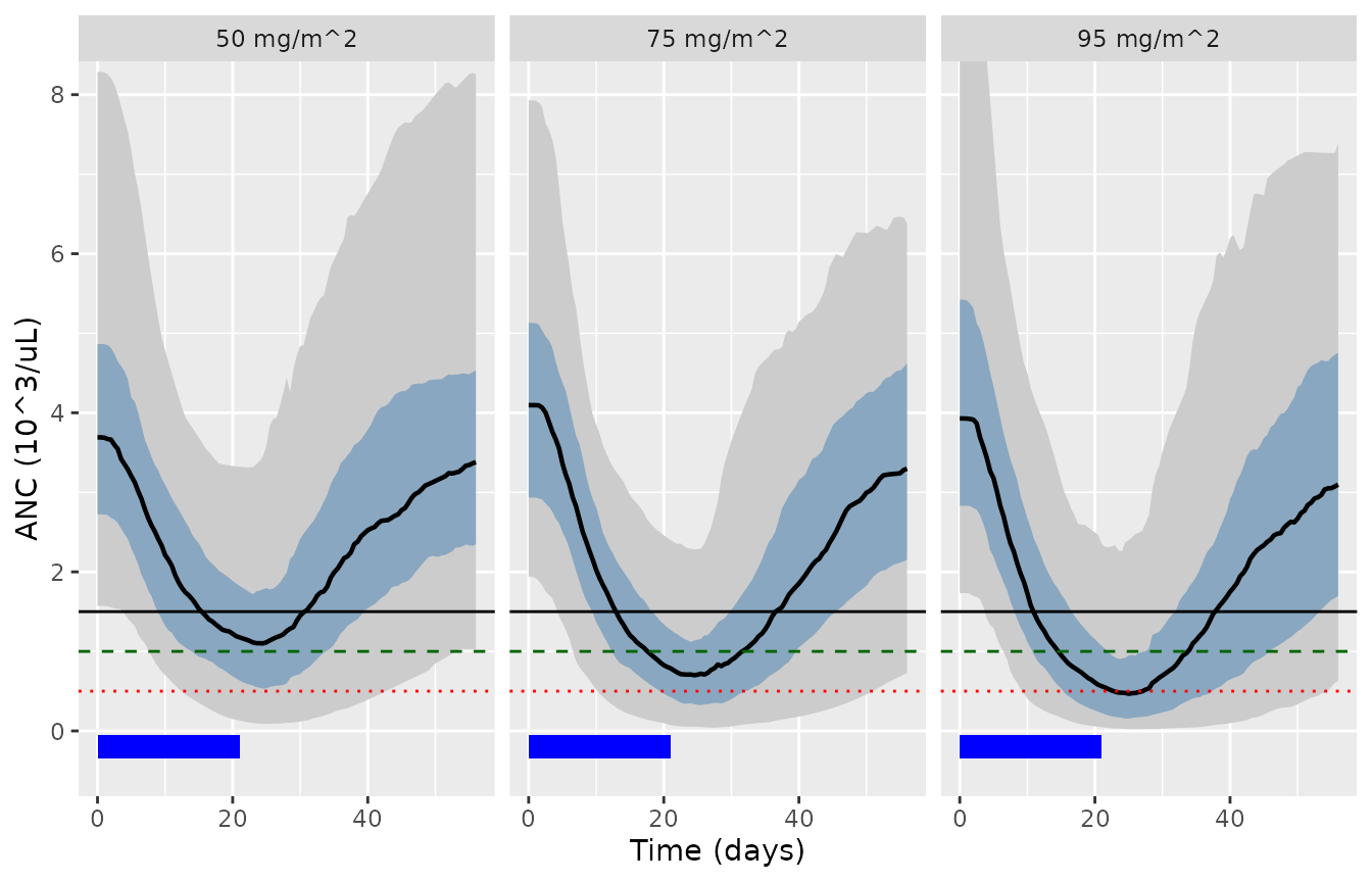
Replicates Figure 4A-C of Panetta 2024: simulated ANC over 56 days after 21 days of daily palbociclib. Horizontal lines are the grade 2, 3 and 4 neutropenia thresholds (1.5, 1.0 and 0.5 x 10^3/uL).
ggplot(band_plt, aes(time)) +
  geom_ribbon(aes(ymin = p05, ymax = p95), fill = "grey80") +
  geom_ribbon(aes(ymin = p25, ymax = p75), fill = "steelblue", alpha = 0.5) +
  geom_line(aes(y = med), linewidth = 0.8) +
  geom_hline(yintercept = 100, linetype = "solid", colour = "black") +
  geom_hline(yintercept = 50, linetype = "dashed", colour = "darkgreen") +
  geom_hline(yintercept = 25, linetype = "dotted", colour = "red") +
  annotate("rect", xmin = 0, xmax = 21, ymin = -18, ymax = -3, fill = "blue") +
  facet_wrap(~dose_label) +
  coord_cartesian(ylim = c(-20, 500)) +
  labs(x = "Time (days)", y = "PLT (10^9/L)")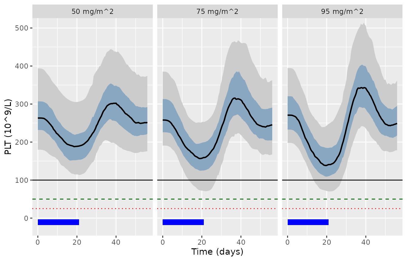
Replicates Figure 4D-F of Panetta 2024: simulated platelet count over 56 days. Horizontal lines are the grade 1, 2 and 3 thrombocytopenia thresholds (100, 50 and 25 x 10^9/L).
The simulated median curves reproduce the published shapes. ANC declines through the dosing period to a nadir a few days after the last dose (typical-value nadir at day 24.0, 24.5 and 25.0 for 50, 75 and 95 mg/m^2, against a last dose on day 20), then recovers – fully by around day 50 at 50 mg/m^2, but only to about 94% and 85% of baseline by day 56 at 75 and 95 mg/m^2, so recovery is still incomplete at the end of the 28-day course at the higher dosages. The platelet count reaches its nadir near the end of dosing (day 18.5-19.5) and rebounds above baseline before settling, peaking at 114-127% of baseline – the overshoot visible in Figure 4D-F, which the bounded feedback term generates.
Replicating Table 4
Table 4 tabulates the proportion of simulated individuals whose nadir falls below each toxicity threshold. Panetta 2024 sampled from the 31 study patients’ individual conditional distributions; the cohorts here are drawn from the population distribution instead, which widens the tails (see Assumptions).
nadir_summary <- function(x, thresholds) {
  x |>
    dplyr::group_by(dose_label, id) |>
    dplyr::summarise(nadir = min(value), .groups = "drop_last") |>
    dplyr::group_by(dose_label) |>
    dplyr::summarise(
      `Median nadir` = round(median(nadir), 2),
      !!paste0("% < ", thresholds[1]) := round(100 * mean(nadir < thresholds[1]), 1),
      !!paste0("% < ", thresholds[2]) := round(100 * mean(nadir < thresholds[2]), 1),
      !!paste0("% < ", thresholds[3]) := round(100 * mean(nadir < thresholds[3]), 1),
      .groups = "drop"
    ) |>
    dplyr::rename(Dosage = dose_label)
}

knitr::kable(nadir_summary(sim_anc, c(1.5, 1.0, 0.5)),
caption = "Simulated ANC nadir (10^3/uL). Panetta 2024 Table 4 reports % below 1.5 / 1.0 / 0.5 of 45 / 19 / 3.1 at 50 mg/m^2, 72 / 49 / 13 at 75 mg/m^2 and 79 / 69 / 32 at 95 mg/m^2.")| Dosage | Median nadir | % < 1.5 | % < 1 | % < 0.5 |
|---|---|---|---|---|
| 50 mg/m^2 | 1.01 | 71.5 | 49.0 | 25.5 |
| 75 mg/m^2 | 0.65 | 84.5 | 72.5 | 42.5 |
| 95 mg/m^2 | 0.43 | 88.5 | 81.5 | 57.0 |
knitr::kable(nadir_summary(sim_plt, c(100, 50, 25)),
caption = "Simulated platelet nadir (10^9/L). Panetta 2024 Table 4 reports % below 100 / 50 / 25 of 6 / 0 / 0 at 50 mg/m^2, 8 / 6 / 0 at 75 mg/m^2 and 12 / 6 / 3 at 95 mg/m^2.")| Dosage | Median nadir | % < 100 | % < 50 | % < 25 |
|---|---|---|---|---|
| 50 mg/m^2 | 186.74 | 1.0 | 0.0 | 0.0 |
| 75 mg/m^2 | 155.47 | 13.5 | 0.5 | 0.0 |
| 95 mg/m^2 | 138.22 | 20.5 | 2.0 | 0.5 |
Read these against Table 4 with the sampling difference in mind; the agreement is good for central tendency and deliberately imperfect in the tails.
- Platelets agree closely. The simulated median nadirs (187, 155 and 138 x 10^9/L) sit just below the published individual-fit median of 169 x 10^9/L (section 3.5), and the proportion below 100 x 10^9/L is the right order of magnitude at every dosage (1, 14 and 21% against 6, 8 and 12%).
- ANC agrees on the median but over-predicts the lower tail. The simulated median nadir at 50 mg/m^2 (1.01 x 10^3/uL) matches the published individual-fit median of 1.0 (section 3.4), but the simulated proportion below 0.5 x 10^3/uL is 25.5% against Table 4’s 3.1%, and the deeper dosages are shifted the same way.
Two things drive the tail difference, and both are consequences of simulating a new virtual cohort rather than re-simulating the study patients:
- Panetta 2024 sampled each of the 31 patients’ conditional distributions. Those are shrunk toward the typical value, so their spread is narrower than a draw from the population distribution by construction.
- These models retain the population PK random effects, and they are
very large –
kahas an IIV standard deviation of 0.87 on the log scale andTlag0.67. The paper instead fixed each patient’s PK to their post hoc estimates. Because the drug effect on proliferation saturates asymmetrically, a wider exposure distribution deepens the lower percentiles more than it raises the upper ones.
Neither is a discrepancy in the encoded parameters: the typical-value nadirs in the next section land where the paper’s own median curves do.
The IC50 unit discrepancy
Table 3 and the Equation 1-5 glossary label IC50 and
C_palbociclib as nM, but the tabulated
values are only self-consistent with the paper’s own PK model and
simulations when read as ng/mL – the unit the PK model
actually produces. Palbociclib is C24H29N7O2, relative molecular mass
447.54 g/mol, so applying the conversion would multiply the driving
concentration by 2.2344.
Three independent checks, all failed by the nM reading:
- Supplementary Figure S2 plots each patient’s model-estimated concentration on a log axis against a left axis labelled nM, and the curves peak around 10^2. This model’s steady-state Cmax at 75 mg/m^2 is 121 ng/mL but 271 nM, so the plotted numbers are the ng/mL values – consistent with the paper having carried its concentrations in ng/mL throughout while labelling them nM.
- Both pharmacodynamic models reproduce Figure 4 at all three dosages under the ng/mL reading and badly over-predict depletion under the nM reading.
- Table 4 reports only 6, 8 and 12% of individuals dropping below 100 x 10^9/L, and only 3.1, 13 and 32% of individuals below 0.5 x 10^3/uL. Both require typical nadirs well above those thresholds; the nM reading puts the typical subject below them at every dosage.
The check below settles it. Both endpoints are simulated at their
typical values (no random effects) under each reading of the tabulated
IC50.
Note the direction of the conversion. The model is driven by
Cc in ng/mL, so reading the tabulated number as nM means
the drug is more potent on that scale:
559.14 nM is only
559.14 / 2.2344 = 250.2 ng/mL. Dividing IC50
by 2.2344 is exactly equivalent to multiplying the driving concentration
by 2.2344, and it predicts deeper depletion than the packaged
reading.
# nM per (ng/mL) for palbociclib, C24H29N7O2, relative molecular mass 447.54.
MW_FACTOR <- 1000 / 447.54

typical_nadir <- function(model, output, ic50_ngml) {
  vapply(c(50, 75, 95), function(d) {
    s <- rxode2::rxSolve(model, pd_events(d), returnType = "data.frame",
                         omega = NA, params = c(lic50 = log(ic50_ngml)))
    min(s[[output]], na.rm = TRUE)
  }, numeric(1))
}

ic50_check <- data.frame(
  Dosage = c("50 mg/m^2", "75 mg/m^2", "95 mg/m^2"),
  `PLT, published curve` = c(205, 175, 160),
  `PLT, ng/mL (packaged)` = round(typical_nadir(mod_plt, "PLT", 559.14), 0),
  `PLT, nM reading` = round(typical_nadir(mod_plt, "PLT", 559.14 / MW_FACTOR), 0),
  `ANC, ng/mL (packaged)` = round(typical_nadir(mod_anc, "ANC", 383.5), 2),
  `ANC, nM reading` = round(typical_nadir(mod_anc, "ANC", 383.5 / MW_FACTOR), 2),
  check.names = FALSE
)
knitr::kable(ic50_check, caption = "Typical-value nadirs under each reading of the tabulated IC50. PLT in 10^9/L, ANC in 10^3/uL. The PLT reference column is read off the median curves of Figure 4D-F.")| Dosage | PLT, published curve | PLT, ng/mL (packaged) | PLT, nM reading | ANC, ng/mL (packaged) | ANC, nM reading |
|---|---|---|---|---|---|
| 50 mg/m^2 | 205 | 191 | 128 | 1.14 | 0.24 |
| 75 mg/m^2 | 175 | 163 | 89 | 0.59 | 0.07 |
| 95 mg/m^2 | 160 | 143 | 67 | 0.36 | 0.03 |
Both endpoints reject the nM reading, and neither is ambiguous:
- Platelets. The packaged reading tracks the published median curves; the nM reading is roughly 40% low at every dosage and puts the typical subject below the 100 x 10^9/L threshold that Table 4 says only 6, 8 and 12% of individuals cross.
- Neutrophils. The packaged reading gives typical nadirs that straddle the Table 4 thresholds in the right places (above 1.0 x 10^3/uL at 50 mg/m^2, where only 19% of individuals fall below it). The nM reading essentially wipes out the circulating pool at every dosage, which is irreconcilable with Table 4 reporting only 3.1, 13 and 32% of individuals below 0.5 x 10^3/uL.
The models therefore use the tabulated numbers with the units read as ng/mL.
Pharmacokinetics and NCA validation
The PK model is validated against the study’s own sampling design: a single oral dose on course 1 day 1 sampled pre-dose and at 0.5, 1, 2, 4, 8, 24 and 48 h, and steady state on course 1 day 21 sampled pre-dose and at 1, 2, 4, 8 and 24 h (section 2.2).
set.seed(20241128L)

pk_single <- rxode2::et(amt = 75, cmt = "depot") |>
  rxode2::et(c(0, 0.5, 1, 2, 4, 8, 24, 48), cmt = "central") |>
  as.data.frame()
pk_single$AST <- 25
pk_single$OCC <- 1

pk_ss <- rxode2::et(amt = 75, cmt = "depot", ii = 24, until = 24 * 20) |>
  rxode2::et(24 * 20 + c(0, 1, 2, 4, 8, 24), cmt = "central") |>
  as.data.frame()
pk_ss$AST <- 25
pk_ss$OCC <- 2

sim_one <- function(ev, treatment, t0) {
  s <- rxode2::rxSolve(mod_pk, ev, nSub = 200, returnType = "data.frame",
                       addDosing = FALSE)
  stopifnot(length(unique(s$sim.id)) == 200L)
  data.frame(id = s$sim.id, time = s$time - t0, Cc = s$Cc, treatment = treatment) |>
    dplyr::filter(!is.na(Cc))
}

pk_conc <- dplyr::bind_rows(
  sim_one(pk_single, "Day 1 (single dose)", 0),
  sim_one(pk_ss, "Day 21 (steady state)", 24 * 20)
)

pk_dose <- pk_conc |>
  dplyr::distinct(id, treatment) |>
  dplyr::mutate(time = 0, amount = 75)

# Same guard as for the pharmacodynamic cohorts: the simulated exposures must
# actually vary between subjects.
stopifnot(
  pk_conc |>
    dplyr::group_by(treatment, id) |>
    dplyr::summarise(cmax = max(Cc), .groups = "drop_last") |>
    dplyr::summarise(cv = sd(cmax) / mean(cmax), .groups = "drop") |>
    dplyr::pull(cv) |> min() > 0.1
)
pk_conc |>
  # The pre-dose record is exactly zero on day 1 and would drop out of a log
  # axis. It is dropped for plotting only; the PKNCA input below keeps it,
  # because the time-zero row is what anchors the AUC interval at 0.
  dplyr::filter(Cc > 0) |>
  dplyr::group_by(treatment, time) |>
  dplyr::summarise(p05 = quantile(Cc, 0.05), med = median(Cc),
                   p95 = quantile(Cc, 0.95), .groups = "drop") |>
  ggplot(aes(time)) +
  geom_ribbon(aes(ymin = p05, ymax = p95), fill = "grey80") +
  geom_line(aes(y = med), linewidth = 0.8) +
  facet_wrap(~treatment, scales = "free_x") +
  scale_y_log10() +
  labs(x = "Time after dose (h)", y = "Palbociclib (ng/mL)")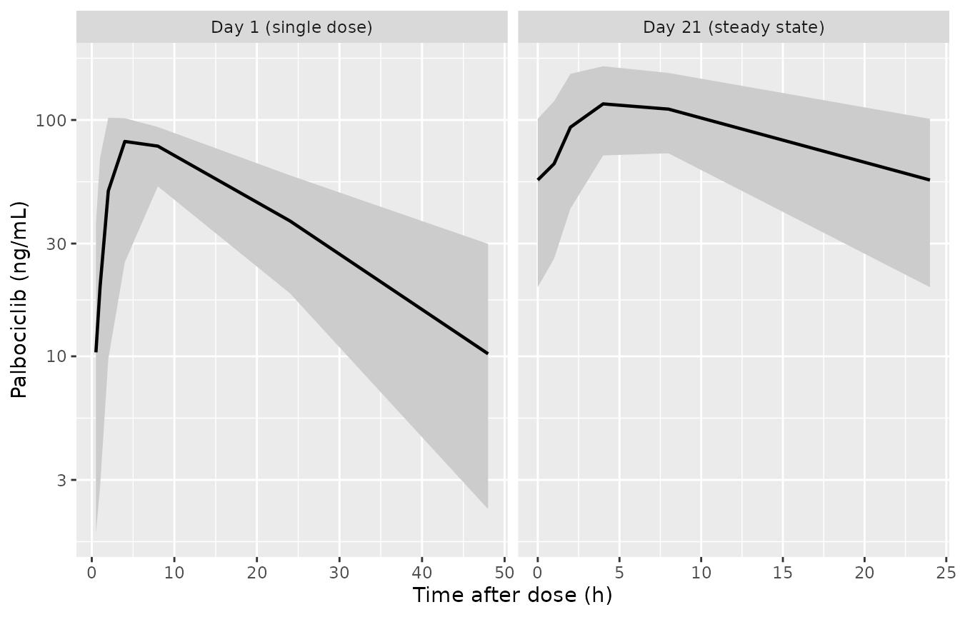
Simulated palbociclib plasma concentrations at 75 mg/m^2. Compare with the prediction-corrected visual predictive checks in Figure 2e (single dose) and 2f (steady state) of Panetta 2024.
conc_obj <- PKNCA::PKNCAconc(pk_conc, Cc ~ time | treatment + id,
                             concu = "ng/mL", timeu = "h")
dose_obj <- PKNCA::PKNCAdose(pk_dose, amount ~ time | treatment + id,
                             doseu = "mg/m^2")

# Only Cmax / Tmax / AUClast are requested here. The study's sampling design is
# too sparse to support lambda-z on a per-subject basis -- the day-21 arm has
# six samples, and in subjects with a long lag or slow absorption only one or
# two of them fall after Tmax -- so asking for half.life / AUCinf per subject
# yields warnings rather than estimates. Those parameters are validated on the
# dense typical-value profile below instead.
intervals <- data.frame(
  start = 0,
  end = c(48, 24),
  treatment = c("Day 1 (single dose)", "Day 21 (steady state)"),
  cmax = TRUE, tmax = TRUE, auclast = TRUE
)

nca <- PKNCA::pk.nca(PKNCA::PKNCAdata(conc_obj, dose_obj, intervals = intervals))
nca_summary <- as.data.frame(nca) |>
  dplyr::filter(!is.na(PPORRES)) |>
  dplyr::group_by(treatment, PPTESTCD) |>
  dplyr::summarise(PPORRES = median(PPORRES), .groups = "drop")
cl.obs needs an explicit unit conversion before it can
be compared with the paper. Doses are in mg/m^2 and concentrations in
ng/mL, so PKNCA returns dose / AUC in mg/m^2 per ng*h/mL;
multiplying by 1000 gives L/h/m^2.
# 1 (mg/m^2)/(ng*h/mL) = 1e6 ng/m^2 / (ng*h/mL) = 1e6 mL/(h*m^2) = 1000 L/(h*m^2)
CL_UNIT_FACTOR <- 1000
Comparison against published values
Panetta 2024 does not tabulate NCA parameters of its own, so the reference column combines the model’s own structural parameters with the pediatric values the paper cites. The paper quotes a Tmax of 5-8 h and a half-life of 11.3-19.5 h from the pediatric phase 1 report (Introduction), and Raetz’s pediatric non-compartmental CL/F of 40.4 L/h/m^2 (section 4).
The clearance check is run on the typical-value
profile over a dense grid rather than on the population median. That
makes it a closed-form identity: non-compartmental
dose / AUC(0-inf) must return the model’s own
CL/F of 36.5 L/h/m^2 exactly. The population median cannot
serve this purpose here, because the very large inter-individual
variability on ka (SD 0.87 on the log scale) drives some
subjects into flip-flop kinetics, where the terminal slope reflects
absorption rather than elimination and AUC(0-inf) is biased
low.
pk_typ <- rxode2::et(amt = 75, cmt = "depot") |>
  rxode2::et(seq(0, 168, by = 0.25), cmt = "central") |>
  as.data.frame()
pk_typ$AST <- 25
pk_typ$OCC <- 1

typ <- rxode2::rxSolve(mod_pk, pk_typ, returnType = "data.frame", omega = NA)
typ_conc <- data.frame(id = 1L, treatment = "Typical value",
                       time = typ$time, Cc = typ$Cc) |>
  dplyr::filter(!is.na(Cc))
typ_dose <- data.frame(id = 1L, treatment = "Typical value",
                       time = 0, amount = 75)

typ_nca <- PKNCA::pk.nca(PKNCA::PKNCAdata(
  PKNCA::PKNCAconc(typ_conc, Cc ~ time | treatment + id,
                   concu = "ng/mL", timeu = "h"),
  PKNCA::PKNCAdose(typ_dose, amount ~ time | treatment + id,
                   doseu = "mg/m^2"),
  intervals = data.frame(start = 0, end = 168, treatment = "Typical value",
                         cmax = TRUE, tmax = TRUE, auclast = TRUE,
                         half.life = TRUE, aucinf.obs = TRUE, cl.obs = TRUE)
))

typ_wide <- as.data.frame(typ_nca) |>
  dplyr::filter(!is.na(PPORRES)) |>
  dplyr::select(treatment, PPTESTCD, PPORRES) |>
  tidyr::pivot_wider(names_from = PPTESTCD, values_from = PPORRES) |>
  dplyr::mutate(cl.obs = cl.obs * CL_UNIT_FACTOR)

# Closed-form identity: AUC(0-inf) must equal Dose / (CL/F).
stopifnot(abs(typ_wide$aucinf.obs - 75 / 36.5 * 1000) < 1)
reference <- data.frame(
  treatment = "Typical value",
  tmax = 6.5,
  half.life = 15.4,
  cl.obs = 36.5
)

cmp <- nlmixr2lib::ncaComparisonTable(
  simulated = dplyr::select(typ_wide, treatment, tmax, half.life, cl.obs),
  reference = reference,
  by = "treatment",
  params = c("tmax", "half.life", "cl.obs"),
  units = c(tmax = "h", half.life = "h", cl.obs = "L/h/m^2")
)
knitr::kable(cmp, caption = "Typical-value single-dose NCA versus reference values. Tmax and half-life references are the midpoints of the 5-8 h and 11.3-19.5 h ranges quoted in the Introduction of Panetta 2024; CL/F is the model's own Table 2 estimate.")| NCA parameter | treatment | Reference | Simulated | % diff |
|---|---|---|---|---|
| Tmax (h) | Typical value | 6.5 | 6 | -7.7% |
| t½ (h) | Typical value | 15.4 | 12.4 | -19.4% |
| CL/F (L/h/m^2) | Typical value | 36.5 | 36.5 | +0.0% |
attr(cmp, "footnote")
#> NULL
The population summary below is descriptive rather than a validation target, for the flip-flop reason given above.
nca_summary |>
  tidyr::pivot_wider(names_from = PPTESTCD, values_from = PPORRES) |>
  dplyr::mutate(dplyr::across(dplyr::any_of("cl.obs"),
                              \(x) x * CL_UNIT_FACTOR)) |>
  dplyr::select(dplyr::any_of(c("treatment", "cmax", "tmax", "auclast",
                                "aucinf.obs", "half.life", "cl.obs"))) |>
  dplyr::rename(Treatment = treatment) |>
  knitr::kable(digits = 2,
caption = "Median simulated NCA parameters at 75 mg/m^2 (200 subjects per arm). AUC is in ng*h/mL, concentrations in ng/mL, Tmax and half-life in h, clearance in L/h/m^2.")| Treatment | cmax | tmax | auclast |
|---|---|---|---|
| Day 1 (single dose) | 86.73 | 8 | 1795.12 |
| Day 21 (steady state) | 122.13 | 4 | 2036.67 |
The AST covariate is checked directly against the two values quoted in section 3.2, which are the only covariate predictions the paper prints.
data.frame(
  `AST (U/L)` = c(10, 25, 100),
  `Published CL/F` = c(48.2, NA, 24.1),
  `Model CL/F` = round(36.5 * (c(10, 25, 100) / 25)^-0.3, 2),
  check.names = FALSE
) |>
knitr::kable(caption = "Apparent oral clearance versus AST (L/h/m^2). Panetta 2024 section 3.2 reports 48.2 at AST = 10 U/L and 24.1 at AST = 100 U/L; 25 U/L is the cohort median at which the power model is centred.")| AST (U/L) | Published CL/F | Model CL/F |
|---|---|---|
| 10 | 48.2 | 48.05 |
| 25 | NA | 36.50 |
| 100 | 24.1 | 24.08 |
Assumptions and deviations
-
IC50 units. Table 3 and the Equation 1-5 glossary
label
IC50andC_palbociclibas nM. The packaged models read the tabulated values as ng/mL, because the nM reading contradicts Supplementary Figure S2, Figure 4 and Table 4 of the same paper. See “The IC50 unit discrepancy” above for the three checks. This is the single largest interpretive decision in this extraction and it changes the predicted depth of myelosuppression by roughly a factor of two. -
The missing
N_PBMfactor in Equation 1. The proliferation term is first-order inN_PBM. This is forced by Equations 6 and 7, not assumed; see “Equation 1 as printed” above. -
k_bpparameterisation. Table 3 tabulatesk_bp(0.78 and 0.52 /day), but sections 2.4.1 and 2.4.2 state that what was actually estimated is the fractionfk_bp = k_bp / kin, on a logit scale, so thatkin > k_bpalways holds. The models encodelogitfktr = qlogis(k_bp / kin)and recoverk_bpasfk_bp * kin. This matters for simulation: with independent log-normal random effects onkinandk_bp, roughly a third of simulated subjects would drawkin < k_bpand get a negative feedback constantK_M. -
fk_bpvariability scale. Table 3 reports thek_bpIIV and IOV as CV%, but a logit-normal parameter has no CV-to-variance identity. The logit-scale standard deviations were obtained with the delta method,sd_logit = CV / (1 - p), and each is round-trip checked in the model file against the published CV. Both are small and poorly estimated in the source (RSE 99-203%). -
Occasion definition. Panetta 2024 reports
inter-occasion variability on CL/F (PK, two sampling visits) and on
kin,k_bpandIC50(PD, courses 1 and 2) but never names an occasion column. The canonicalOCCcovariate is used, with two occasions. In the PD models the PK inter-occasion term is keyed to the same course index; the PK analysis’s own occasions were the course 1 day 1 and day 21 visits, about three weeks apart and so comparable in span to a treatment course. SetOCC = 1throughout for a single-occasion simulation. - Base versus final PK model. The Abstract quotes the base-model estimates (V/F 664.5 L/m^2, CL/F 36.8 L/h/m^2, ka 0.48 /h). The packaged models use the AST column of Table 2, which is the final model that Figure 2’s diagnostics and the bootstrap refer to.
-
PK residual error in the PD models. The PD models
were fitted with the pharmacokinetics fixed to individual post hoc
estimates, so their likelihood contains only the blood-count residual
error.
Ccis therefore exposed in the PD models as a derived variable with no error model; the plasma residual error lives inPanetta_2024_palbociclib. - PK inter-individual variability retained in the PD models. The PD fit used each patient’s own post hoc PK parameters. For simulation the population PK random effects are retained so that a virtual cohort has realistic exposure variability.
- Simulation cohorts. Panetta 2024 simulated by sampling each of the 31 study patients’ conditional distributions (n = 10 per patient). The cohorts here are drawn from the population distribution, which has wider tails because it is not shrunk toward the typical value, and they retain the large population PK random effects that the paper replaced with individual post hoc estimates. Central tendency agrees closely (see “Replicating Table 4”), but the simulated ANC lower tail is materially heavier than Table 4 – 25.5% below 0.5 x 10^3/uL at 50 mg/m^2 against the published 3.1%. Treat the tail percentiles of this vignette as a property of the virtual cohort, not as a reproduction of Table 4.
- NCA reference values. Panetta 2024 reports no NCA table of its own. The Tmax and half-life references are midpoints of the 5-8 h and 11.3-19.5 h ranges quoted in the Introduction from the pediatric phase 1 report, and are therefore approximate.
- No BSA covariate. Doses are in mg/m^2 and volumes and clearances are per m^2, so BSA cancels exactly. This reproduces the paper’s own model input convention rather than adding a scaling covariate.