Angiotensin challenge dose-response (Buchwalder-Csajka 1999)
Source:vignettes/articles/BuchwalderCsajka_1999_angiotensin.Rmd
BuchwalderCsajka_1999_angiotensin.RmdModel and source
- Citation: Buchwalder-Csajka C, Buclin T, Brunner HR, Biollaz J. Evaluation of the angiotensin challenge methodology for assessing the pharmacodynamic profile of antihypertensive drugs acting on the renin-angiotensin system. Br J Clin Pharmacol. 1999 Oct;48(4):594-604. doi:10.1046/j.1365-2125.1999.00050.x
- Description: Population pharmacodynamic dose-response model of the peak systolic (SBP) and diastolic (DBP) blood pressure increase elicited by a single intravenous bolus of exogenous angiotensin (used as a pharmacologic probe / ‘challenge’) in 228 healthy male volunteers across 13 phase I trials of antihypertensive drugs acting on the renin-angiotensin system. The final structural form is the molecular-weight-corrected Emax model E = Emax * D / (D + ED50) (Buchwalder-Csajka 1999 Table 1 last row), where D = DOSE_AGT_UG is the angiotensin challenge dose in ug already expressed as angiotensin II equivalents (multiply an angiotensin I dose by Q = 0.78 in data preparation; the paper’s text reports Q = 0.78 as the molar-weight ratio), and Emax / ED50 are estimated separately for SBP and DBP. This is a purely algebraic snapshot model: no PK, no time course, no ODEs. Each observation row in the event dataset carries one DOSE_AGT_UG value (the dose given just before the peak was sampled) and yields one peak BP increase. The model is suitable for simulating the peak BP response to a single angiotensin bolus during dose-finding and placebo-period segments of an angiotensin-challenge phase I protocol; it is NOT a model of the antihypertensive drugs whose trials supplied the data.
- Article: Br J Clin Pharmacol 48:594-604 (1999)
This is a purely algebraic population pharmacodynamic snapshot model. There is no PK, no time course, and no ODE. Each observation row in the event table represents one challenge: an intravenous bolus of angiotensin given to a healthy volunteer, and the peak systolic (SBP) and diastolic (DBP) blood pressure increase recorded immediately afterward by a non-invasive Finapres servo-photoplethysmomanometer. The model predicts the peak BP increase as an Emax function of the dose:
E = Emax * D / (D + ED50)
where D is the dose expressed in ug of angiotensin II equivalents (DOSE_AGT_UG in the event table). Q = 0.78 (Ang I -> Ang II molar-weight conversion) is applied during data preparation rather than inside the model. PKNCA-based NCA validation does not apply because there is no concentration-time course; instead this vignette compares typical-value model predictions to the published Table 1 estimates and abstract claims, and replicates the Figure 1 individual peak-response cloud.
Population
228 healthy male volunteers participated in the 13 phase I trials that contributed to the analysis (Buchwalder-Csajka 1999 Methods, p. 595). 1144 angiotensin-induced peaks were used to fit the dose-response model. Figure 1 of the source paper shows individual dose-response curves for the 185-subject subset that received both angiotensin I and angiotensin II challenges. All volunteers were male (Methods p. 596); the source paper reports that age, body weight, height, and ethnic group had no detectable influence on the dose-response relationship over the range of subjects studied, so the final model carries no demographic covariates. The challenges modeled here are the exogenous angiotensin boluses given during dose-finding and placebo periods, NOT the antihypertensive drugs under investigation in those trials.
The same metadata is available programmatically via the model’s
population field
(rxode2::rxode(readModelDb("BuchwalderCsajka_1999_angiotensin"))$population).
Source trace
The per-parameter origin is recorded as an in-file comment next to
each ini() entry in
inst/modeldb/specificDrugs/BuchwalderCsajka_1999_angiotensin.R.
The table below collects them in one place.
| Equation / parameter | Value | Source location |
|---|---|---|
Structural form E = Emax * D / (D + ED50) with Q
correction baked into D |
n/a | Table 1 last row; Results “Angiotensin dose-response relationship” (p. 596-597) |
lemax_dbp -> Emax_DBP |
36.7 mmHg | Table 1 row 5 DBP column |
lemax_sbp -> Emax_SBP |
40.9 mmHg | Table 1 row 5 SBP column |
led50_dbp -> ED50_DBP |
0.80 ug Ang II eq. | Table 1 row 5 DBP column |
led50_sbp -> ED50_SBP |
0.65 ug Ang II eq. | Table 1 row 5 SBP column |
| Q (Ang I -> Ang II molar conversion) | 0.78 (fixed; baked into DOSE_AGT_UG, not estimated inside the model) | Methods (p. 595, paragraph after the model equations); Results “Angiotensin dose-response relationship” (p. 596-597) |
etalemax_dbp (paper SD 4.8 mmHg, additive) |
omega2_log = 0.0170 | Table 1 row 5 DBP +/-; Methods “a_j = a + eta_a” (p. 595) |
etalemax_sbp (paper SD 6.6 mmHg, additive) |
omega2_log = 0.0258 | Table 1 row 5 SBP +/-; Methods (p. 595) |
etaled50_dbp (paper SD 0.3 ug, additive) |
omega2_log = 0.1315 | Table 1 row 5 DBP +/-; Methods (p. 595) |
etaled50_sbp (paper SD 0.4 ug, additive) |
omega2_log = 0.3149 | Table 1 row 5 SBP +/-; Methods (p. 595) |
addSd_dbp |
4.2 mmHg | Table 1 row 5 DBP Se column |
addSd_sbp |
5.2 mmHg | Table 1 row 5 SBP Se column |
| Population n (volunteers) | 228 | Methods “Angiotensin dose-response relationship” (p. 595) |
| Observations n (peaks) | 1144 | Methods (p. 595) |
| Trials n | 13 | Methods (first paragraph, p. 595) |
Virtual cohort
The original peak-by-peak data are not publicly available. The vignette uses a virtual population of 185 subjects (matching the Figure 1 sample size), each receiving a spread of angiotensin doses across the 0.5-5 ug Ang II equivalents range observed in the paper.
set.seed(19990929)

# Doses on a log spacing -- matches the log-x-axis of Figure 1.
dose_grid <- exp(seq(log(0.5), log(5), length.out = 7))
dose_grid <- round(dose_grid, 3)
dose_grid
#> [1] 0.500 0.734 1.077 1.581 2.321 3.406 5.000

n_subjects <- 185L

events <- expand.grid(
  id          = seq_len(n_subjects),
  DOSE_AGT_UG = dose_grid
) |>
  dplyr::arrange(id, DOSE_AGT_UG) |>
  dplyr::group_by(id) |>
  dplyr::mutate(time = seq_len(dplyr::n()) - 1L) |>
  dplyr::ungroup() |>
  dplyr::mutate(evid = 0L, amt = 0)

head(events)
#> # A tibble: 6 × 5
#>      id DOSE_AGT_UG  time  evid   amt
#>   <int>       <dbl> <int> <int> <dbl>
#> 1     1       0.5       0     0     0
#> 2     1       0.734     1     0     0
#> 3     1       1.08      2     0     0
#> 4     1       1.58      3     0     0
#> 5     1       2.32      4     0     0
#> 6     1       3.41      5     0     0
nrow(events)
#> [1] 1295
Simulation
mod <- readModelDb("BuchwalderCsajka_1999_angiotensin")

# Stochastic simulation with IIV: per-subject eta values sample once
# at the subject level and persist across all of that subject's
# dose rows, so individual subjects produce smooth dose-response
# curves (matching the Figure 1 panel structure).
sim <- rxode2::rxSolve(mod, events = events, keep = c("DOSE_AGT_UG"))
#> ℹ parameter labels from comments will be replaced by 'label()'
sim_df <- as.data.frame(sim)

# Typical-value (no-IIV) curves for the overlay.
mod_typical <- rxode2::zeroRe(mod)
#> ℹ parameter labels from comments will be replaced by 'label()'
typical_dose_grid <- exp(seq(log(0.4), log(6), length.out = 50))
typical_events <- data.frame(
  id          = 1L,
  time        = seq_along(typical_dose_grid) - 1L,
  evid        = 0L,
  amt         = 0,
  DOSE_AGT_UG = typical_dose_grid
)
typical_sim <- as.data.frame(rxode2::rxSolve(
  mod_typical, events = typical_events, keep = c("DOSE_AGT_UG")
))
#> ℹ omega/sigma items treated as zero: 'etalemax_dbp', 'etalemax_sbp', 'etaled50_dbp', 'etaled50_sbp'
Replicate published figures
Figure 1 – individual peak DBP responses
Buchwalder-Csajka 1999 Figure 1 plots individual peak diastolic BP responses for 185 healthy subjects against the angiotensin challenge dose, on a log-spaced x-axis spanning roughly 0.4 to 6 ug Ang II equivalents, with the average log-linear and Emax population curves overlaid (lower panel). The simulated cloud below uses the packaged Emax model. The curve is the typical-value Emax fit; the thin lines are individual subjects sampled from the population IIV.
ggplot() +
  geom_line(
    data = sim_df,
    aes(x = DOSE_AGT_UG, y = dbp, group = id),
    alpha = 0.15
  ) +
  geom_line(
    data = typical_sim,
    aes(x = DOSE_AGT_UG, y = dbp),
    colour = "firebrick", linewidth = 1.1
  ) +
  scale_x_log10(breaks = c(0.4, 0.8, 1.6, 3.2, 6.4)) +
  labs(
    x = "Angiotensin dose (ug Ang II equivalents)",
    y = "Peak DBP increase (mmHg)",
    title = "Figure 1 (DBP panel) -- individual peak DBP responses",
    caption = "Replicates Figure 1 of Buchwalder-Csajka 1999 (lower panel, Emax model). Thin lines: 185 simulated subjects. Red: typical-value Emax curve."
  ) +
  theme_minimal()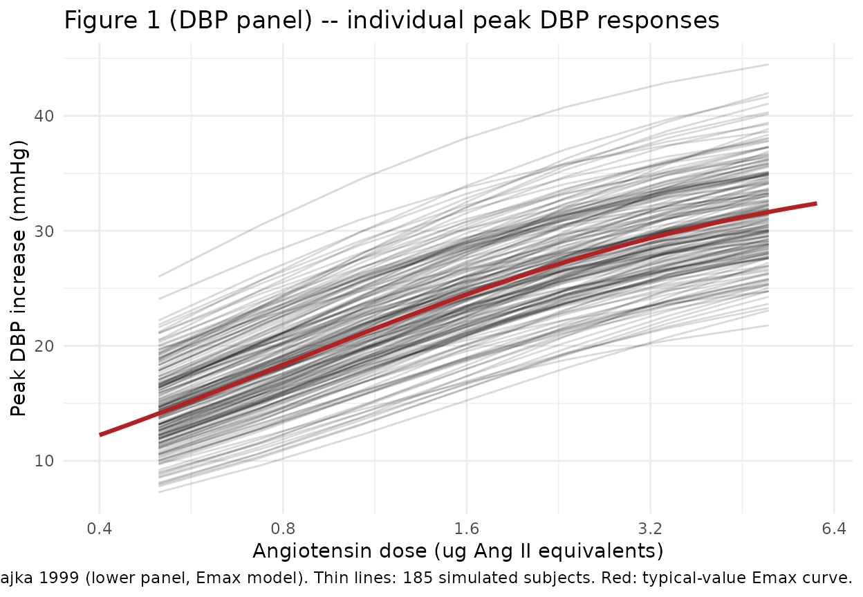
Figure 1 – typical-value Emax curve for SBP and DBP
The two-output structure produces parallel Emax curves for SBP and DBP.
typical_long <- typical_sim |>
  dplyr::select(DOSE_AGT_UG, sbp, dbp) |>
  tidyr::pivot_longer(c(sbp, dbp), names_to = "endpoint", values_to = "delta_BP")

ggplot(typical_long, aes(DOSE_AGT_UG, delta_BP, colour = endpoint)) +
  geom_line(linewidth = 1.1) +
  scale_x_log10(breaks = c(0.4, 0.8, 1.6, 3.2, 6.4)) +
  labs(
    x = "Angiotensin dose (ug Ang II equivalents)",
    y = "Typical peak BP increase (mmHg)",
    colour = "Endpoint",
    title = "Typical-value Emax dose-response, SBP and DBP",
    caption = "SBP curve approaches Emax = 40.9 mmHg; DBP curve approaches Emax = 36.7 mmHg."
  ) +
  theme_minimal()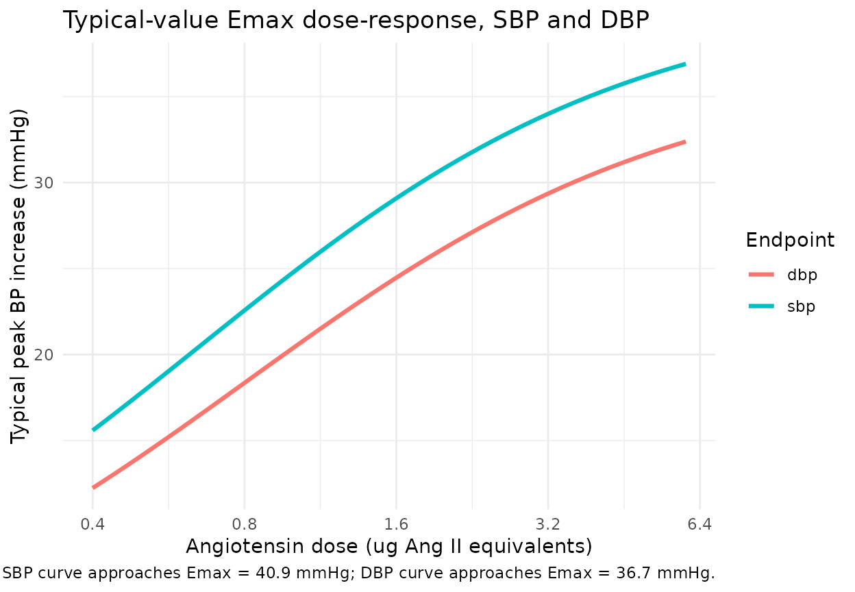
Validation against published estimates
The Buchwalder-Csajka 1999 abstract reports “an average systolic/diastolic response of 24 +/- 6/20 +/- 5 mmHg for a unit dose of 1 ug of angiotensin II equivalents” from the log-linear model fit. The Emax model produces nearly identical typical-value predictions at 1 ug (the log-linear and Emax fits agree closely on the ascending limb of the dose-response curve; the paper notes the dose range only covered the inferior ascending part of the curve, p. 597).
unit_dose_events <- data.frame(
  id          = 1L,
  time        = 0L,
  evid        = 0L,
  amt         = 0,
  DOSE_AGT_UG = 1.0
)
unit_dose_pred <- as.data.frame(rxode2::rxSolve(
  mod_typical, events = unit_dose_events, keep = c("DOSE_AGT_UG")
))
#> ℹ omega/sigma items treated as zero: 'etalemax_dbp', 'etalemax_sbp', 'etaled50_dbp', 'etaled50_sbp'

unit_dose_pred[, c("DOSE_AGT_UG", "sbp", "dbp")]
#>   DOSE_AGT_UG      sbp      dbp
#> 1           1 24.78788 20.38889
Side-by-side comparison of the simulated typical predictions, the abstract’s log-linear claim, and the Table 1 row 5 Emax point estimates:
mod_ui <- rxode2::rxode(readModelDb("BuchwalderCsajka_1999_angiotensin"))
#> ℹ parameter labels from comments will be replaced by 'label()'
ini_lookup <- function(name) {
  row <- mod_ui$iniDf[mod_ui$iniDf$name == name, , drop = FALSE]
  row$est
}
emax_dbp_typ <- exp(ini_lookup("lemax_dbp"))
emax_sbp_typ <- exp(ini_lookup("lemax_sbp"))

comparison <- tibble::tribble(
  ~Quantity,                                          ~`Simulated typical (Emax)`, ~`Paper abstract (log-linear at 1 ug)`, ~`Paper Table 1 row 5 (Emax with Q)`,
  "DBP peak at 1 ug Ang II equivalents (mmHg)",       round(unit_dose_pred$dbp, 2), "20 +/- 5",                              "Emax = 36.7 +/- 4.8; ED50 = 0.8 +/- 0.3 ug",
  "SBP peak at 1 ug Ang II equivalents (mmHg)",       round(unit_dose_pred$sbp, 2), "24 +/- 6",                              "Emax = 40.9 +/- 6.6; ED50 = 0.65 +/- 0.4 ug",
  "Asymptotic DBP peak (Emax_DBP, mmHg)",             round(emax_dbp_typ, 2),       "n/a",                                   "36.7",
  "Asymptotic SBP peak (Emax_SBP, mmHg)",             round(emax_sbp_typ, 2),       "n/a",                                   "40.9"
)
knitr::kable(comparison, caption = "Typical-value predictions vs Buchwalder-Csajka 1999 Table 1 / abstract.")| Quantity | Simulated typical (Emax) | Paper abstract (log-linear at 1 ug) | Paper Table 1 row 5 (Emax with Q) |
|---|---|---|---|
| DBP peak at 1 ug Ang II equivalents (mmHg) | 20.39 | 20 +/- 5 | Emax = 36.7 +/- 4.8; ED50 = 0.8 +/- 0.3 ug |
| SBP peak at 1 ug Ang II equivalents (mmHg) | 24.79 | 24 +/- 6 | Emax = 40.9 +/- 6.6; ED50 = 0.65 +/- 0.4 ug |
| Asymptotic DBP peak (Emax_DBP, mmHg) | 36.70 | n/a | 36.7 |
| Asymptotic SBP peak (Emax_SBP, mmHg) | 40.90 | n/a | 40.9 |
At 1 ug the Emax model predicts SBP / DBP peaks of about 24.8 / 20.4 mmHg, well within the additive 1-SD of the abstract’s log-linear quotes of 24 +/- 6 / 20 +/- 5 mmHg.
Stochastic dose-response summary
Quantile summary across the 185-subject virtual cohort confirms the population-scale spread implied by the packaged log-normal IIV.
sim_summary <- sim_df |>
  dplyr::group_by(DOSE_AGT_UG) |>
  dplyr::summarise(
    dbp_p05 = round(quantile(dbp, 0.05), 2),
    dbp_p50 = round(quantile(dbp, 0.50), 2),
    dbp_p95 = round(quantile(dbp, 0.95), 2),
    sbp_p05 = round(quantile(sbp, 0.05), 2),
    sbp_p50 = round(quantile(sbp, 0.50), 2),
    sbp_p95 = round(quantile(sbp, 0.95), 2),
    .groups = "drop"
  )
knitr::kable(sim_summary, caption = "Simulated 5th / 50th / 95th percentiles by angiotensin dose, n = 185 virtual subjects.")| DOSE_AGT_UG | dbp_p05 | dbp_p50 | dbp_p95 | sbp_p05 | sbp_p50 | sbp_p95 |
|---|---|---|---|---|---|---|
| 0.500 | 9.03 | 14.35 | 20.43 | 8.83 | 17.48 | 29.93 |
| 0.734 | 11.67 | 17.71 | 24.04 | 11.66 | 21.33 | 33.72 |
| 1.077 | 14.70 | 21.17 | 27.95 | 14.68 | 25.29 | 37.14 |
| 1.581 | 17.91 | 24.45 | 31.66 | 18.35 | 28.75 | 39.89 |
| 2.321 | 20.89 | 27.14 | 34.48 | 21.20 | 31.56 | 42.15 |
| 3.406 | 23.47 | 29.50 | 36.39 | 24.54 | 34.06 | 44.94 |
| 5.000 | 25.28 | 31.41 | 38.56 | 27.24 | 36.31 | 46.66 |
Assumptions and deviations
IIV reparameterisation – log-normal vs additive. The source paper specifies the random effect additively on the natural scale (
a_j = a + eta_a,b_j = b + eta_b; Methods p. 595). The packaged model log-transforms Emax and ED50 for positivity (following theZhou_2016_warfarin_vk2lemax/lec50/lic50precedent) and converts the paper’s additive SD to a log-normal omega^2 viaomega2_log = log(1 + (SD / mean)^2). The typical-value point estimates (exp(lemax) = paper Emax) are unchanged. The IIV distribution shape is a near-exact match for the small-CV Emax parameters (CV ~13-16%) and a mild approximation at the higher ED50 CVs (~38-62%), where the log-normal sides higher than the additive form on the upper tail but rules out the negative-ED50 region that the paper’s additive parameterisation would otherwise admit.Q = 0.78 conversion baked into DOSE_AGT_UG. The paper applies Q = 0.78 inside the structural model, with the dose being either the literal Ang II mass or the Ang I mass multiplied by Q. The packaged model expects DOSE_AGT_UG already in Ang II equivalents, so the Q conversion is a data-preparation step (multiply Ang I doses by 0.78 before populating DOSE_AGT_UG). This is mathematically equivalent and keeps the rxode2 model free of a categorical “ang type” switch.
Log-linear alternative not packaged. Table 1 also reports a log-linear fit (
E = a * ln(D * Q) + b, witha = 8.5 / 9.1andb = 20.2 / 24.5mmHg for DBP / SBP). The paper notes that the log-linear form was “thought to give more adequate estimates” because the dose range did not cover the upper plateau, but the Emax form had the lower objective function (OF 4778 / 5342 vs 4769 / 5490 – OF improvement of 9 SBP units). Both reasonably describe the ascending portion of the dose-response. The packaged model uses the Emax fit because that is the lowest-OF final form in Table 1 and because the abstract emphasises ED50 values from the Emax fit. The log-linear alternative is reproducible by hand from the Table 1 row-3 estimates if downstream users need it.Demographic covariates intentionally absent. The paper screened age, body weight, height, and ethnic group (with all volunteers being male, so sex was not assessable) and reported none of them influencing the dose-response over the range studied (Methods p. 595 + Results “Angiotensin dose-response relationship”, p. 596-597). No demographic covariate is packaged. The Buchwalder-Csajka 1999 study population is reflected in the
populationmetadata; downstream users who wish to add a covariate must rely on a different (likely external) source.No PK / no time course. The angiotensin challenge response is treated as an instantaneous peak following the bolus; the paper’s upstream dose-finding protocol established that each subject’s characteristic peak occurs at a similar post-bolus interval, and the peak is the only quantity modeled. There is no concentration-time curve to compare against, so PKNCA validation is intentionally absent from this vignette; the validation is instead the side-by-side comparison of typical predictions against Table 1 / abstract above.
Errata search. A search for corrigenda or errata on Br J Clin Pharmacol vol. 48 against Buchwalder-Csajka 1999 returned no published corrections at the time of extraction; all values are taken from the primary article as published.