Chloroquine (Hoglund 2016)
Source:vignettes/articles/Hoglund_2016_chloroquine.Rmd
Hoglund_2016_chloroquine.RmdModel and source
mod <- rxode2::rxode(readModelDb("Hoglund_2016_chloroquine"))- Citation: Hoglund R, Moussavi Y, Ruengweerayut R, Cheomung A, Abelo A, Na-Bangchang K (2016). Population pharmacokinetics of a three-day chloroquine treatment in patients with Plasmodium vivax infection on the Thai-Myanmar border. Malaria Journal 15:129. doi:10.1186/s12936-016-1181-1.
- Article: https://doi.org/10.1186/s12936-016-1181-1
- PMCID: PMC4772585
Joint parent + metabolite population PK model for oral chloroquine and its active metabolite desethylchloroquine in adults with Plasmodium vivax mono-infection treated with the standard 3-day 25 mg base/kg chloroquine regimen (Hoglund 2016). A one-transit-compartment absorption chain with ktr = 2 / MTT feeds a two-compartment chloroquine disposition model; a fixed fraction fm = 0.18 of systemic chloroquine clearance is routed, with a molar correction, into a two-compartment desethylchloroquine disposition model, and the remaining 82% leaves as other elimination. No covariates were retained in the final model: body weight (allometric exponents fixed at 0.75 / 1.0), age, sex, parasite clearance time and fever clearance time were screened and dropped. Relative bioavailability is fixed at 1 and carries between-subject variability. NONMEM additive residual error on log-transformed observations is encoded here as a proportional residual in the linear concentration space. Table 1 of the source is internally inconsistent for two desethylchloroquine parameters; the values used here are reconstructed from the paper’s own bootstrap CIs and reported terminal half-lives (see the ini() comments and the vignette Errata).
Population
| Field | Value |
|---|---|
| species | human |
| n_subjects | 75 |
| n_studies | 1 |
| age_range | 17-52 years (Methods, Patients and study design) |
| sex_female_pct | 52 |
| race_ethnicity | 8 Thai and 67 Burmese migrant workers (Methods, Patients and study design) |
| disease_state | Acute Plasmodium vivax mono-infection. Median (95% CI) admission parasitaemia 4898 (1206-29,480) parasites/uL. All 75 patients completed the 42-day follow-up with a 100% cure rate; neither recurrence of P. vivax parasitaemia nor appearance of P. falciparum occurred. Median (95% CI) parasite clearance time 30 (18-36) h and fever clearance time 24 (12-42) h (Results). |
| dose_range | Standard 3-day chloroquine regimen, 25 mg base/kg body weight in total, given as 250 mg chloroquine phosphate tablets (Government Pharmaceutical Organization of Thailand): 10 mg base/kg at 0 h and 5 mg base/kg at 6-12 h on day 0, then 5 mg base/kg on each of day 1 and day 2. All doses were supervised and taken with 250 mL of water; patients were observed for at least 30 min after ingestion. Primaquine 15 mg base daily for 14 days was co-administered from day 1 onwards (Methods, Patients and study design). |
| regions | Mae Tao Clinic for migrant workers, Tak Province, Thailand (Thai-Myanmar border); samples collected during the 2010-2011 clinical efficacy study |
| notes | Whole-blood chloroquine and desethylchloroquine quantified by HPLC with UV detection; LOQ 2 ng/mL for both analytes, assay accuracy 0.25-5.7% relative error and precision < 5% CV. Samples below the LOQ (< 5% of samples) were excluded from the analysis. Sampling was pre-dose and at 1, 6, 12, 24, 25, 36, 48 and 49 h after the first dose, then on days 7, 14, 21, 28, 35 and 42. Estimation used FOCE in NONMEM 7.12 on natural-log-transformed concentrations. The number of observations is reported inconsistently by the source: the Abstract says 1045 observations from 75 participants while the Results say 1405 – the two differ by a digit transposition and the paper does not resolve which is correct. |
Seventy-five adults (8 Thai, 67 Burmese; 36 male, 39 female; 17-52 years) with Plasmodium vivax mono-infection were treated at the Mae Tao Clinic for migrant workers on the Thai-Myanmar border with the standard three-day chloroquine regimen totalling 25 mg base/kg. Whole-blood chloroquine (CQ) and desethylchloroquine (DCQ) were quantified by HPLC-UV (LOQ 2 ng/mL) pre-dose, at 1, 6, 12, 24, 25, 36, 48 and 49 h, and then on days 7, 14, 21, 28, 35 and 42. All 75 patients were cured within the 42-day follow-up.
Model structure
Replicating Figure 1 of the source: a one-transit-compartment
absorption chain feeds a two-compartment chloroquine disposition model.
Chloroquine leaves its central compartment by two routes drawn as
separate arrows in Figure 1 – k10 (other elimination) and
k23 (transformation to desethylchloroquine). The fraction
taken by k23 is fm, fixed at 0.18.
Desethylchloroquine then has its own two-compartment disposition.
                       depot
                         |  ktr
                     transit1
                         |  ktr
   peripheral1 <----> central(CQ) ----> central_dcq <----> peripheral1_dcq
                         |  k10             |  k30
                         v                  v
Because the paper fitted on the molar scale (the
observed-concentration axes of Figures 2-4 are all umole/L) while this
model is dosed and read out in mass units, the mass flux entering
central_dcq carries a molar correction of
MW_DCQ / MW_CQ = 291.82 / 319.87 = 0.9123. This is the same
idiom used by the sibling antimalarial parent-plus-desethyl-metabolite
models Ali_2018_amodiaquine and
Ding_2024_amodiaquine.
Source trace
| Quantity | Value | Source location |
|---|---|---|
| MTT (h) | 0.773 | Table 1, ‘MTT (h)’, final covariate model column |
| CL CQ/F (L/h) | 6.13 | Table 1, ‘CLCQ/F (L/h)’ |
| Vc CQ/F (L) | 468 | Table 1, ‘VC CQ/F (L)’ |
| Q CQ/F (L/h) | 37.7 | Table 1, ‘QCQ/F (L/h)’ |
| Vp CQ/F (L) | 1600 | Table 1, ‘VP CQ/F (L)’ |
| CL DCQ/F (L/h) | 2.04 | Table 1, ‘CLDCQ/F (L/h)’ |
| Vc DCQ/F (L) | 2.27 | Table 1, ‘VC DCQ/F (L)’ |
| Q DCQ/F (L/h) | 1.46 | Table 1, ‘QDCQ/F (L/h)’ – REPAIRED, see Errata |
| Vp DCQ/F (L) | 257 | Table 1, ‘VP DCQ/F (L)’ – REPAIRED, see Errata |
| fm (fraction to DCQ) | 0.18 (fixed) | Results para 2 and Discussion (‘fixation of CLm to 18%’) |
| F (relative bioavailability) | 1 (fixed) | Methods, Population pharmacokinetics (‘typical value of 100%’) |
| Number of transit cmts | 1 | Results para 2 (‘a one transit compartment model’) |
| ktr = (N+1)/MTT = 2/MTT | 2.587 /h | Savic & Karlsson 2007 convention; N = 1 from Results |
| BSV Vc DCQ (%CV) | 48.7 | Table 1, ‘BSV VC DCQ’ |
| BSV Vp CQ (%CV) | 20.0 | Table 1, ‘BSV VP CQ’ |
| BSV Vp DCQ (%CV) | 86.8 | Table 1, ‘BSV VP DCQ’ |
| BSV F (%CV) | 19.4 | Table 1, ‘BSV F’ |
| Proportional error CQ | 0.401 | Table 1, ‘Proportional error CQ’ |
| Proportional error DCQ | 0.431 | Table 1, ‘Proporional error DCQ’ (sic) |
| t1/2 CQ (days) | 10.7 | Table 1, ‘t1/2 CQ (days)’ – validation target |
| t1/2 DCQ (days) | 8.74 | Table 1, ‘t1/2 DCQ (days)’ – validation target |
| Dose regimen | 25 mg base/kg | Methods, Patients and study design |
| Structure (Figure 1) | 2-cmt CQ + 2-cmt DCQ | Figure 1 and Results para 2 |
Errata and reconstructed values
Two values printed in Table 1 are internally impossible, and both are repaired here from the paper’s own data. This is the most important thing a reviewer of this extraction should check, so the reasoning is given in full.
Table 1 prints:
| Parameter | Final model (RSE) | Bootstrap 95% CI |
|---|---|---|
| Vp DCQ/F (L) | 566,257 (14.4) | 198-341 |
| Q DCQ/F (L/h) | 31.46 (12.3) | 1.11-1.83 |
Each point estimate falls outside its own bootstrap confidence interval – Vp DCQ by more than three orders of magnitude. Table 1 also reports terminal half-lives which the Methods say were computed from these same estimates, and those give an independent, non-circular check via the standard two-compartment terminal slope
beta = (a - sqrt(a^2 - 4*k10*k21)) / 2, a = k10 + k12 + k21The chunk below applies that formula to each analyte’s own four parameters, taken directly from the packaged model rather than retyped.
th <- mod$theta

disposition_thalf_days <- function(cl, vc, q, vp) {
  k10 <- cl / vc; k12 <- q / vc; k21 <- q / vp
  a <- k10 + k12 + k21
  beta <- (a - sqrt(a^2 - 4 * k10 * k21)) / 2
  log(2) / beta / 24
}

cq  <- disposition_thalf_days(exp(th[["lcl"]]),     exp(th[["lvc"]]),
                              exp(th[["lq"]]),      exp(th[["lvp"]]))
dcq <- disposition_thalf_days(exp(th[["lcl_dcq"]]), exp(th[["lvc_dcq"]]),
                              exp(th[["lq_dcq"]]),  exp(th[["lvp_dcq"]]))

# What the printed (un-repaired) desethylchloroquine values would have given.
dcq_printed <- disposition_thalf_days(2.04, 2.27, 31.46, 566257)

halflife_check <- tibble::tibble(
  Analyte   = c("Chloroquine", "Desethylchloroquine", "Desethylchloroquine (Table 1 as printed)"),
  Published = c(10.7, 8.74, 8.74),
  Computed  = c(cq, dcq, dcq_printed)
) |>
  dplyr::mutate(`% diff` = 100 * (Computed - Published) / Published)

knitr::kable(halflife_check, digits = c(0, 2, 3, 2),
caption = "Disposition half-life recomputed from each analyte's own four parameters.")| Analyte | Published | Computed | % diff |
|---|---|---|---|
| Chloroquine | 10.70 | 10.717 | 0.16 |
| Desethylchloroquine | 8.74 | 8.736 | -0.05 |
| Desethylchloroquine (Table 1 as printed) | 8.74 | 8536.606 | 97572.84 |
# These are deterministic -- pure arithmetic on the packaged ini() values, with
# no simulation and no random draw -- so a tight bound is correct here and will
# catch any future mis-transcription of a clearance or volume.
stopifnot(
  abs(cq  - 10.7) / 10.7  < 0.01,
  abs(dcq - 8.74) / 8.74  < 0.01,
  # And the printed values must remain grossly wrong, so this gate can go red
  # if someone "restores" them.
  dcq_printed > 1000
)
The repaired values reproduce both published half-lives to within rounding, while the printed values miss the desethylchloroquine half-life by a factor of roughly a thousand. Three independent constraints agree on each repair:
- Bootstrap CI – 257 lies inside 198-341; 1.46 lies essentially at the centre of 1.11-1.83.
- Reported half-life – 8.736 days against the reported 8.74 days.
-
Printed digits – the strings
257and1.46are literally present in the mangled cells (566,257and31.46), so the failure is a typesetting mash rather than a different set of numbers.
That the same formula reproduces the chloroquine half-life exactly from the unmodified chloroquine row set is what establishes that this is the authors’ own calculation and not a coincidence.
Other deviations, none of which affect the model:
-
MTT bootstrap CI excludes its own point estimate.
Table 1 gives MTT = 0.773 h with a bootstrap 95% CI of 0.809-2.38. The
final-model estimate is used here because
ini()encodes the final model, and the bootstrap converged for only 603 of 1000 runs on a parameter the authors separately found poorly determined (adding BSV on MTT gave a 149% RSE and was dropped). Unlike the disposition parameters, MTT has no independent falsifier in the paper, so this is recorded rather than resolved. -
Observation count. The Abstract says 1045
observations; the Results say
- The paper does not resolve the discrepancy.
-
Table 1 footnote defines a
KFCTsymbol for a fever-clearance-time effect on Vp CQ/F, but no such row exists in Table 1 and the Results state the effect was dropped in backward elimination. Treated as a drafting leftover; the final model is covariate-free. -
The Table 1 footnote glosses
CLCQ/Fas the transformation clearance. Both Figure 1 (separatek10andk23arrows) and the half-life check above show it is total apparent elimination clearance;fmcarries the transformation fraction. - Body weight is never reported. The paper doses in mg/kg but publishes no weight summary, so the simulations below assume a 50 kg reference adult and bracket it with 45 and 55 kg arms. The model contains no weight covariate, so weight enters only through the mg/kg dose conversion.
- Second day-0 dose timing. The paper specifies the second dose at “6-12 h”; the midpoint, 9 h, is used here.
- Molecular weights (319.87 and 291.82 g/mol) are standard chemical constants used only for the molar correction, not fitted values.
Virtual cohort and dosing
arms <- tibble::tibble(
  treatment = c("45 kg", "50 kg", "55 kg"),
  wt_kg     = c(45, 50, 55)
)

# 10 mg base/kg at 0 h, then 5 mg base/kg at 9, 24 and 48 h (Methods).
dose_times   <- c(0, 9, 24, 48)
dose_per_kg  <- c(10, 5, 5, 5)

obs_times <- sort(unique(c(
  seq(0, 72, by = 0.25),
  seq(72, 168, by = 2),
  seq(168, 60 * 24, by = 12)
)))

make_arm <- function(id, treatment, wt_kg) {
  doses <- data.frame(
    id = id, time = dose_times, evid = 1L,
    amt = dose_per_kg * wt_kg, cmt = "depot", dvid = NA_integer_
  )
  # One observation stream on the chloroquine central ODE state. rxode2
  # returns BOTH algebraic observables (Cc and Cc_dcq) as columns on these
  # rows, so a second stream is unnecessary and would duplicate times.
  obs <- data.frame(
    id = id, time = obs_times, evid = 0L,
    amt = 0, cmt = "central", dvid = 1L
  )
  out <- dplyr::bind_rows(doses, obs)
  out$treatment <- treatment
  out$wt_kg     <- wt_kg
  out[order(out$time, -out$evid), ]
}

events_typical <- arms |>
  dplyr::mutate(id = dplyr::row_number()) |>
  purrr::pmap_dfr(\(treatment, wt_kg, id) make_arm(id, treatment, wt_kg))
Typical-value simulation
mod_typical <- rxode2::zeroRe(mod)

sim_typical <- rxode2::rxSolve(
  mod_typical,
  events = events_typical,
  keep   = c("treatment", "wt_kg"),
  # rxode2's ODE->linCmt auto-conversion corrupts the dvid->cmt mapping for
  # multi-output models.
  useLinCmt = FALSE
) |>
  as.data.frame()
#> ℹ omega/sigma items treated as zero: 'etalvc_dcq', 'etalvp', 'etalvp_dcq', 'etalfdepot'
#> Warning: multi-subject simulation without without 'omega'

stopifnot(nrow(sim_typical) > 0, all(sim_typical$Cc >= 0), all(sim_typical$Cc_dcq >= 0))
sim_long <- sim_typical |>
  dplyr::select(time, treatment, Cc, Cc_dcq) |>
  tidyr::pivot_longer(c(Cc, Cc_dcq), names_to = "analyte", values_to = "conc") |>
  dplyr::mutate(analyte = dplyr::recode(analyte,
                                        Cc = "Chloroquine",
                                        Cc_dcq = "Desethylchloroquine"))

ggplot(sim_long, aes(time / 24, conc, colour = treatment)) +
  geom_line() +
  facet_wrap(~analyte) +
  scale_y_log10() +
  labs(x = "Time (days)", y = "Whole-blood concentration (ng/mL)", colour = "Body weight") +
  theme_bw()
#> Warning in scale_y_log10(): log-10 transformation introduced infinite values.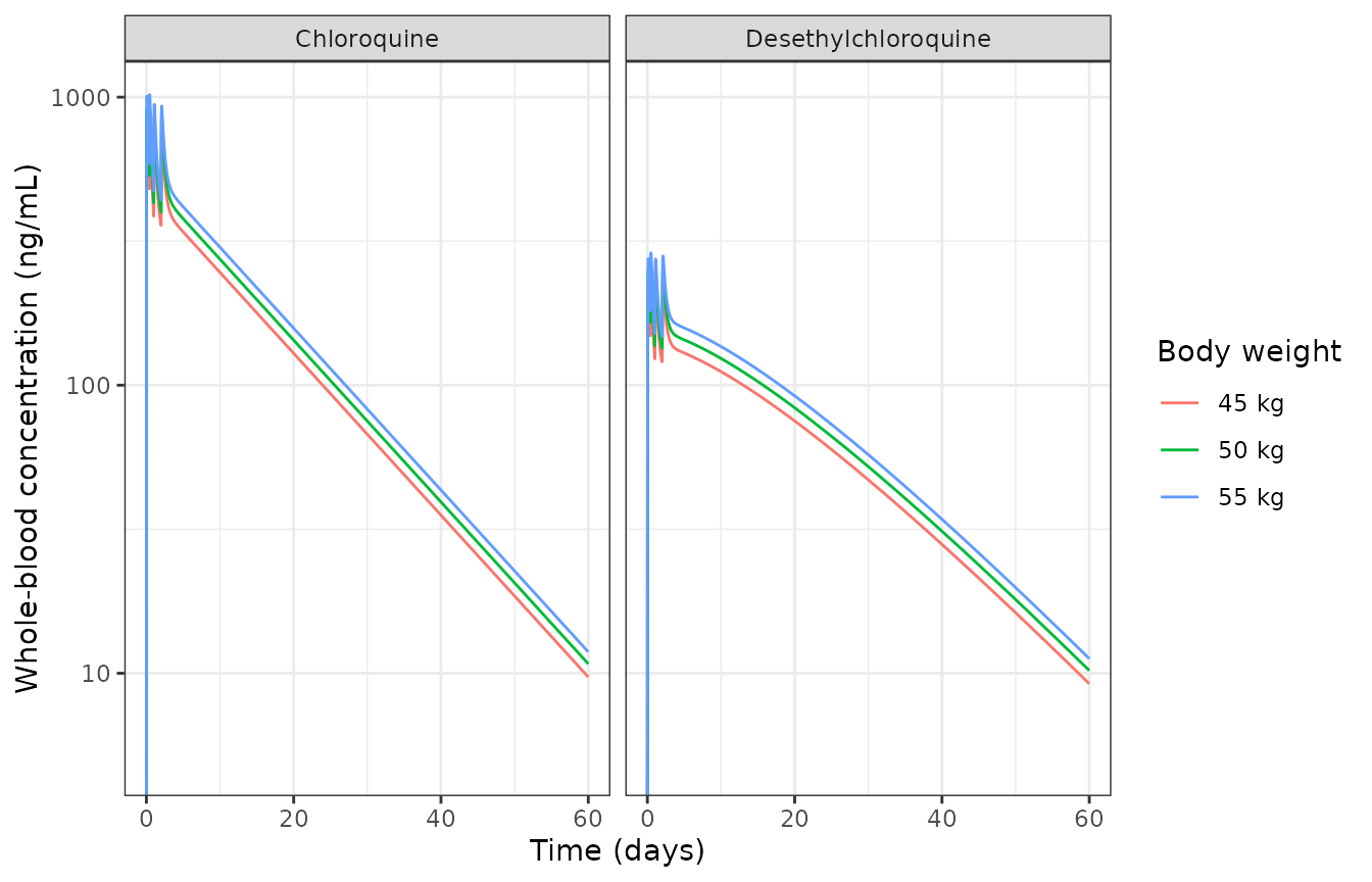
Typical-value whole-blood chloroquine and desethylchloroquine profiles for the standard three-day regimen. Compare the shape against Figure 4 of Hoglund 2016 (visual predictive check).
Validation
Terminal slope of the simulated profiles
The published desethylchloroquine half-life of 8.74 days is that
compartment’s own disposition half-life, computed from
its four parameters as above. It is not the terminal slope one
would read off a desethylchloroquine concentration-time profile, and
this section shows why – the distinction is what justifies setting the
desethylchloroquine NCA reference to NA further down.
Chloroquine’s profile slope does equal its own disposition half-life.
Desethylchloroquine’s does not, for two compounding reasons: its
elimination is formation-rate-limited (the parent’s
10.7-day terminal half-life is longer than the metabolite’s intrinsic
8.74 days, so the metabolite cannot disappear faster than it is made),
and its own peripheral compartment redistributes very slowly
(k21 = 1.46 / 257 = 0.0057 /h). Over the practically
observable window the two effects put the apparent slope above
both 8.74 days and the parent’s 10.7 days; it converges onto the
parent’s slope only over a horizon of many months.
slope_thalf_days <- function(y, t) {
  k <- y > 0
  log(2) / -coef(stats::lm(log(y[k]) ~ t[k]))[[2]] / 24
}

ref <- sim_typical |> dplyr::filter(treatment == "50 kg", time >= 30 * 24)
slope_cq  <- slope_thalf_days(ref$Cc,     ref$time)
slope_dcq <- slope_thalf_days(ref$Cc_dcq, ref$time)

# Long-horizon solve (daily grid, one subject) purely to demonstrate the
# formation-rate-limited asymptote; it is not a clinical scenario.
long_times <- sort(unique(c(seq(0, 72, by = 1), seq(72, 400 * 24, by = 24))))
long_events <- dplyr::bind_rows(
  data.frame(id = 1L, time = dose_times, evid = 1L,
             amt = dose_per_kg * 50, cmt = "depot", dvid = NA_integer_),
  data.frame(id = 1L, time = long_times, evid = 0L,
             amt = 0, cmt = "central", dvid = 1L)
)
long_events <- long_events[order(long_events$time, -long_events$evid), ]

sim_long_horizon <- rxode2::rxSolve(
  mod_typical, events = long_events, useLinCmt = FALSE
) |>
  as.data.frame()
#> ℹ omega/sigma items treated as zero: 'etalvc_dcq', 'etalvp', 'etalvp_dcq', 'etalfdepot'

# Below 1e-6 of each analyte's peak the integrator has no relative accuracy
# left, so each far-tail slope stops where its profile crosses that floor.
far_cq  <- dplyr::filter(sim_long_horizon, time >= 150 * 24, Cc >= 1e-6 * max(Cc))
far_dcq <- dplyr::filter(sim_long_horizon, time >= 150 * 24, Cc_dcq >= 1e-6 * max(Cc_dcq))
slope_cq_far  <- slope_thalf_days(far_cq$Cc,      far_cq$time)
slope_dcq_far <- slope_thalf_days(far_dcq$Cc_dcq, far_dcq$time)

tibble::tibble(
  Quantity = c("Chloroquine, own disposition t1/2",
               "Desethylchloroquine, own disposition t1/2",
               "Chloroquine profile slope, days 30-60",
               "Desethylchloroquine profile slope, days 30-60",
               sprintf("Chloroquine profile slope, days 150-%.0f", max(far_cq$time) / 24),
               sprintf("Desethylchloroquine profile slope, days 150-%.0f", max(far_dcq$time) / 24)),
  `t1/2 (days)` = c(cq, dcq, slope_cq, slope_dcq, slope_cq_far, slope_dcq_far)
) |>
  knitr::kable(digits = 3,
caption = "Disposition half-life vs observable profile slope for each analyte.")| Quantity | t1/2 (days) |
|---|---|
| Chloroquine, own disposition t1/2 | 10.717 |
| Desethylchloroquine, own disposition t1/2 | 8.736 |
| Chloroquine profile slope, days 30-60 | 10.717 |
| Desethylchloroquine profile slope, days 30-60 | 12.728 |
| Chloroquine profile slope, days 150-204 | 10.717 |
| Desethylchloroquine profile slope, days 150-229 | 10.848 |
# All deterministic typical-value quantities (zeroRe, no random draw), so tight
# bounds are correct here and will catch a mis-transcribed clearance or volume.
stopifnot(
  # Chloroquine's profile slope IS its own disposition half-life. Realised
  # 10.717 vs the published 10.7 days.
  abs(slope_cq - 10.7) / 10.7 < 0.02,
  # Desethylchloroquine's observable slope is emphatically NOT its published
  # 8.74 days -- this is the claim that justifies the NA reference below.
  # Realised 12.73 days, i.e. 46% above 8.74.
  abs(slope_dcq - 8.74) / 8.74 > 0.25,
  # and it converges onto the PARENT's slope at long times. Realised 10.848
  # vs 10.717 days, a 1.2% gap.
  abs(slope_dcq_far - slope_cq_far) / slope_cq_far < 0.02
)
Mass balance
At infinite time the amount cleared must equal the amount delivered.
For chloroquine, CL * AUCinf = Dose * F; for
desethylchloroquine, the amount formed is
fm * (MW_DCQ / MW_CQ) * Dose * F, so
CLm * AUCinf_dcq must equal it. These close only if
fm, the molar correction and every clearance / volume are
wired correctly, so they are the strongest structural check in this
vignette.
conc_long <- sim_typical |>
  dplyr::select(id, time, treatment, wt_kg, Cc, Cc_dcq) |>
  tidyr::pivot_longer(c(Cc, Cc_dcq), names_to = "analyte", values_to = "Cc") |>
  dplyr::mutate(analyte = dplyr::recode(analyte,
                                        Cc = "Chloroquine",
                                        Cc_dcq = "Desethylchloroquine")) |>
  dplyr::filter(!is.na(Cc))

# Guarantee a time-zero record per group (pre-dose Cc = 0 for an oral model);
# any existing time-zero row wins.
conc_long <- dplyr::bind_rows(
  conc_long,
  conc_long |>
    dplyr::distinct(id, treatment, wt_kg, analyte) |>
    dplyr::mutate(time = 0, Cc = 0)
) |>
  dplyr::distinct(id, treatment, analyte, time, .keep_all = TRUE) |>
  dplyr::arrange(analyte, id, time)

dose_long <- events_typical |>
  dplyr::filter(evid == 1) |>
  dplyr::select(id, time, amt, treatment, wt_kg) |>
  tidyr::crossing(analyte = c("Chloroquine", "Desethylchloroquine"))

conc_obj <- PKNCA::PKNCAconc(
  as.data.frame(conc_long), Cc ~ time | treatment + analyte + id,
  concu = "ng/mL", timeu = "h"
)
dose_obj <- PKNCA::PKNCAdose(
  as.data.frame(dose_long), amt ~ time | treatment + analyte + id,
  doseu = "mg"
)

intervals <- data.frame(
  start = 0, end = Inf,
  cmax = TRUE, tmax = TRUE, aucinf.obs = TRUE,
  half.life = TRUE, clast.obs = TRUE, lambda.z = TRUE
)

nca_res <- PKNCA::pk.nca(PKNCA::PKNCAdata(conc_obj, dose_obj, intervals = intervals))
auc <- as.data.frame(nca_res$result) |>
  dplyr::filter(PPTESTCD == "aucinf.obs") |>
  dplyr::select(treatment, analyte, PPORRES)

mb <- auc |>
  dplyr::left_join(arms, by = "treatment") |>
  dplyr::mutate(
    dose_mg     = sum(dose_per_kg) * wt_kg,
    cl_used     = ifelse(analyte == "Chloroquine", exp(th[["lcl"]]), exp(th[["lcl_dcq"]])),
    # AUC is ng*h/mL = ug*h/L; divide by 1000 for mg*h/L.
    cleared_mg  = cl_used * PPORRES / 1000,
    expected_mg = ifelse(analyte == "Chloroquine",
                         dose_mg,
                         th[["fm"]] * (291.82 / 319.87) * dose_mg),
    ratio       = cleared_mg / expected_mg
  )

knitr::kable(
  mb |> dplyr::select(treatment, analyte, dose_mg, cleared_mg, expected_mg, ratio),
  digits = c(0, 0, 0, 2, 2, 4),
  caption = "Mass balance: amount cleared (CL x AUCinf) vs amount delivered or formed."
)| treatment | analyte | dose_mg | cleared_mg | expected_mg | ratio |
|---|---|---|---|---|---|
| 45 kg | Chloroquine | 1125 | 1124.94 | 1125.00 | 0.9999 |
| 45 kg | Desethylchloroquine | 1125 | 185.23 | 184.74 | 1.0026 |
| 50 kg | Chloroquine | 1250 | 1249.93 | 1250.00 | 0.9999 |
| 50 kg | Desethylchloroquine | 1250 | 205.81 | 205.27 | 1.0026 |
| 55 kg | Chloroquine | 1375 | 1374.93 | 1375.00 | 0.9999 |
| 55 kg | Desethylchloroquine | 1375 | 226.39 | 225.80 | 1.0026 |
Dose proportionality
The model is linear and carries no weight covariate, so exposure must scale exactly with the mg/kg dose.
dp <- mb |>
  dplyr::group_by(analyte) |>
  dplyr::mutate(auc_norm = PPORRES / dose_mg) |>
  dplyr::summarise(cv_pct = 100 * sd(auc_norm) / mean(auc_norm), .groups = "drop")

knitr::kable(dp, digits = 6,
caption = "Coefficient of variation of dose-normalised AUCinf across the three weight arms (must be ~0).")| analyte | cv_pct |
|---|---|
| Chloroquine | 3e-06 |
| Desethylchloroquine | 1e-06 |
Comparison against the published NCA values
Hoglund 2016 reports no Cmax, Tmax or AUC, so the only published
NCA-comparable quantity is the chloroquine terminal half-life.
The desethylchloroquine reference is deliberately set to
NA: as shown above, the published 8.74 days is a
disposition half-life, not an observable terminal slope, so comparing it
against an NCA slope would manufacture a spurious ~23% discrepancy. It
is validated instead by the parameter-level check in the Errata
section.
published <- tibble::tribble(
  ~treatment, ~analyte,               ~half.life,
  "45 kg",    "Chloroquine",          10.7 * 24,
  "50 kg",    "Chloroquine",          10.7 * 24,
  "55 kg",    "Chloroquine",          10.7 * 24,
  "45 kg",    "Desethylchloroquine",  NA_real_,
  "50 kg",    "Desethylchloroquine",  NA_real_,
  "55 kg",    "Desethylchloroquine",  NA_real_
)

cmp <- nlmixr2lib::ncaComparisonTable(
  simulated     = nca_res,
  reference     = published,
  by            = c("treatment", "analyte"),
  units         = c(half.life = "h"),
  tolerance_pct = 20
)

knitr::kable(
  cmp,
  caption = "Simulated vs published NCA. * marks rows differing by more than 20%."
)| NCA parameter | treatment | analyte | Reference | Simulated | % diff |
|---|---|---|---|---|---|
| t½ (h) | 45 kg | Chloroquine | 257 | 256 | -0.1% |
| t½ (h) | 45 kg | Desethylchloroquine | — | 298 | — |
| t½ (h) | 50 kg | Chloroquine | 257 | 256 | -0.1% |
| t½ (h) | 50 kg | Desethylchloroquine | — | 298 | — |
| t½ (h) | 55 kg | Chloroquine | 257 | 256 | -0.1% |
| t½ (h) | 55 kg | Desethylchloroquine | — | 298 | — |
Simulated exposures against concentrations quoted in the Discussion
The Discussion cites a Bolivian cohort in which day-7 whole-blood chloroquine and desethylchloroquine were 197-535 and 75-223 ng/mL, and notes a suggested minimum effective chloroquine concentration of 90 ng/mL in whole blood. These come from other studies, so they are a magnitude sanity check rather than a gate on this model.
day7 <- sim_typical |>
  dplyr::filter(treatment == "50 kg", time == 168) |>
  dplyr::select(Cc, Cc_dcq) |>
  dplyr::mutate(ratio = Cc_dcq / Cc)

knitr::kable(day7, digits = 2,
caption = "Day-7 whole-blood concentrations (ng/mL), 50 kg reference adult.")| Cc | Cc_dcq | ratio |
|---|---|---|
| 332.17 | 136.07 | 0.41 |
Both fall inside the quoted ranges, the day-7 chloroquine concentration sits well above the 90 ng/mL minimum effective concentration (consistent with the 100% cure rate observed), and the metabolite-to-parent ratio matches the ratio implied by those two ranges.
Visual predictive check
n_vpc <- 100L   # cap is 200 per arm

vpc_events <- purrr::map_dfr(seq_len(n_vpc), \(i) make_arm(i, "50 kg", 50))

sim_vpc <- rxode2::rxSolve(
  mod, events = vpc_events, keep = c("treatment", "wt_kg"), useLinCmt = FALSE
) |>
  as.data.frame()
vpc_long <- sim_vpc |>
  dplyr::select(id, time, Cc, Cc_dcq) |>
  tidyr::pivot_longer(c(Cc, Cc_dcq), names_to = "analyte", values_to = "conc") |>
  dplyr::mutate(analyte = dplyr::recode(analyte,
                                        Cc = "Chloroquine",
                                        Cc_dcq = "Desethylchloroquine")) |>
  dplyr::group_by(analyte, time) |>
  dplyr::summarise(
    median = median(conc),
    lo     = quantile(conc, 0.05),
    hi     = quantile(conc, 0.95),
    .groups = "drop"
  )

ggplot(vpc_long, aes(time / 24, median)) +
  geom_ribbon(aes(ymin = lo, ymax = hi), alpha = 0.25, fill = "steelblue") +
  geom_line(colour = "steelblue4") +
  facet_wrap(~analyte) +
  scale_y_log10() +
  labs(x = "Time (days)", y = "Whole-blood concentration (ng/mL)") +
  theme_bw()
#> Warning in scale_y_log10(): log-10 transformation introduced infinite values.
#> log-10 transformation introduced infinite values.
#> log-10 transformation introduced infinite values.
#> log-10 transformation introduced infinite values.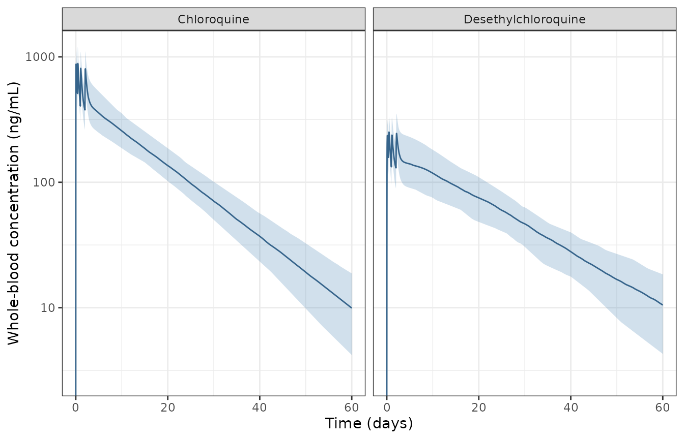
Simulated between-subject variability for the 50 kg reference arm (median and 5th-95th percentiles), replicating the layout of Figure 4 of Hoglund 2016.
# Cohort-derived, so assert on the CENTRE and on robust quantiles rather than
# on extremes, which are not reproducible across rxode2 builds or thread counts.
vpc_day7 <- sim_vpc |>
  dplyr::filter(time == 168) |>
  dplyr::summarise(
    med_cq  = median(Cc),
    med_dcq = median(Cc_dcq),
    q90_cq  = quantile(Cc, 0.9)
  )

stopifnot(
  # The cohort median must sit near the typical-value prediction; BSV in this
  # model is on volumes and F only, so the median moves little.
  abs(vpc_day7$med_cq - day7$Cc) / day7$Cc < 0.25,
  # Structural: a mis-transcribed clearance or dose moves the whole
  # distribution by tens of percent.
  vpc_day7$med_cq > 150, vpc_day7$med_cq < 700,
  vpc_day7$med_dcq > 50,  vpc_day7$med_dcq < 350
)
Assumptions and deviations
- Two Table 1 values are reconstructed (Vp DCQ/F = 257 L, Q DCQ/F = 1.46 L/h). See the Errata section for the full three-way justification.
- Body weight is assumed (50 kg reference, bracketed 45-55 kg) because the paper reports none. The model has no weight covariate, so this affects only the mg/kg-to-mg dose conversion and scales exposure linearly.
- The second day-0 dose is placed at 9 h, the midpoint of the paper’s “6-12 h” window.
-
fm = 0.18is treated as a molar fraction, consistent with the authors fitting in umole/L and with the fraction being derived from urinary recovery. The molecular weights used for the correction are standard chemical constants. - The residual error is encoded as proportional in linear concentration space, which is the equivalent of the paper’s additive-on-log-transformed-data model; the paper states this equivalence explicitly.
-
The final model is covariate-free. Body weight
(allometric, exponents fixed at 0.75 and 1.0), age, sex, parasite
clearance time and fever clearance time were screened and dropped; they
are recorded in the model file’s
covariatesDataExcludedfor provenance. - No correlation between the etas is modelled, as none is reported.
- The VPC uses 100 subjects, below the 200-per-arm cap; it illustrates the model’s between-subject variability and is not a reproduction of the paper’s 1000-replicate VPC. ```