Amoxicillin, levofloxacin and moxifloxacin non-adherence in community-acquired pneumonia (Carral 2023)
Source:vignettes/articles/Carral_2023_cap_nonadherence.Rmd
Carral_2023_cap_nonadherence.RmdModel and source
Carral et al. (2023) used three population PK simulation models to compare how forgiving oral amoxicillin (1000 mg every 8 h), levofloxacin (750 mg once daily) and moxifloxacin (400 mg once daily) are to delayed or missed doses in adult men with community-acquired pneumonia caused by Streptococcus pneumoniae. Each model is given as a NONMEM simulation control stream in the paper’s appendices and is packaged here as its own model:
-
Carral_2023_amoxicillin: One-compartment population PK simulation model for oral amoxicillin in virtual adult male outpatients with community-acquired pneumonia (Carral 2023). Parallel first-order (depot) and lagged zero-order (central) absorption, with the zero-order arm’s bioavailability falling with dose as KD / (KD + DOSE); apparent clearance proportional to Cockcroft-Gault creatinine clearance (CL/F = CL_slope * CLcr / 102) and apparent volume proportional to body weight. The paper’s own Monte Carlo simulation model for adherence / relative-forgiveness analysis, built from the Sjovall data. -
Carral_2023_levofloxacin: Two-compartment population PK simulation model for oral levofloxacin in virtual adult male outpatients with community-acquired pneumonia (Carral 2023). First-order absorption; micro-constant parameterisation in which apparent clearance is a linear regression on Cockcroft-Gault creatinine clearance (computed from ideal body weight) and age, central volume and k21 are linear in age. Reparameterised by the authors from the Preston 1998 demographic model for their Monte Carlo adherence / relative-forgiveness analysis. -
Carral_2023_moxifloxacin: Two-compartment population PK simulation model for oral moxifloxacin in virtual adult male outpatients with community-acquired pneumonia (Carral 2023). First-order absorption; CL/F and Q/F scale with (LBM/60)^0.75 and V2/F and V3/F linearly with lean body mass. Taken by the authors from the Grosjean and Urien 2012 population model for their Monte Carlo adherence / relative-forgiveness analysis. - Citation: Carral N, Lukas JC, Estrade O, Jauregizar N, Morillas H, Suarez E. Non-Adherence in Adult Male Patients with Community-Acquired Pneumonia: Relative Forgiveness of Amoxicillin versus Respiratory Fluoroquinolones. Antibiotics (Basel). 2023;12(5):838. doi:10.3390/antibiotics12050838
- Article (open access): https://doi.org/10.3390/antibiotics12050838
- Supplement (Tables S1 and S2): https://www.mdpi.com/article/10.3390/antibiotics12050838/s1
The amoxicillin model was developed by the authors from the Sjovall et al. data. The levofloxacin model is the authors’ reparameterisation of the Preston et al. (1998) demographic model, and the moxifloxacin model is the Grosjean and Urien (2012) model (Methods 4.2 and 4.3).
Population
No patients were studied. The virtual population is adult Caucasian men aged 31 to 65 years and weighing 70 kg, split into three renal-function subgroups by serum creatinine (0.7, 0.9 and 1.3 mg/dL). Cockcroft-Gault creatinine clearance in the three subgroups is 131 +/- 10, 100 +/- 8 and 70 +/- 6 mL/min (Methods 4.1; Supplementary Tables S1 and S2). Moxifloxacin clearance does not depend on creatinine clearance, so moxifloxacin was simulated as a single group spanning 70-131 mL/min. Each regimen ran for 10 days, and the delayed or missed dose fell on day 4. The paper simulated 10,000 virtual patients per subgroup in NONMEM 7.4.3. This vignette uses 200 per subgroup and scenario.
Two S. pneumoniae susceptibility settings were studied: high susceptibility (PHS, MIC 0.064 mg/L for all three drugs) and low susceptibility (PLS, MIC 1 mg/L for amoxicillin and levofloxacin, 0.25 mg/L for moxifloxacin). The efficacy targets are free time above the MIC for at least 50% of the dosing interval (fT50% >= MIC) for amoxicillin and free AUC0-24h / MIC >= 33.8 for the fluoroquinolones. The unbound fractions are 0.82 for amoxicillin, 0.69 for levofloxacin and 0.52 for moxifloxacin (Methods 4.2 and 4.3).
The same information is available programmatically, for example
readModelDb("Carral_2023_amoxicillin")()$population.
Source trace
All three control streams run in NONMEM ONLYSIM mode, so
the $THETA values are the simulation models’ typical
values. None were re-estimated in this paper. Numeric constants that the
streams write as literals in $PK (regression slopes and the
allometric exponent) are wrapped in fixed().
| Model | Parameter / equation | Value | Source location |
|---|---|---|---|
| Amoxicillin | lka |
log(0.635) 1/h | Appendix A THETA(1) |
| Amoxicillin |
lcl (CL/F at CLcr = 102 mL/min) |
log(15.5) L/h | Appendix A THETA(2); Methods 4.2 |
| Amoxicillin |
lvc (V/F per kg) |
log(0.33) L/kg | Appendix A THETA(3), TVV = THETA(3) * SIMWT |
| Amoxicillin | ALAG1 (first-order arm) | 0 (fixed, omitted) | Appendix A THETA(4) ‘(0 FIXED)’ |
| Amoxicillin | logitffo |
log(0.177) | Appendix A THETA(5); F1 = 1 - 1/(1 + THETA(5)) |
| Amoxicillin | ld2 |
log(1.44) h | Appendix A THETA(6) |
| Amoxicillin |
ltlag (zero-order arm lag) |
log(0.190) h | Appendix A THETA(7); ALAG2 = ALAG1 + THETA(7) |
| Amoxicillin |
led50 (KD) |
log(1300) mg | Appendix A THETA(8); DF = 1 - DOSE/(KD + DOSE) |
| Amoxicillin |
etalka, etalcl, etalvc,
etaled50
|
0.04, 0.036, 0.01, 0.04 | Appendix A $OMEGA ETA(1)-ETA(4) |
| Amoxicillin |
propSd, addSd
|
sqrt(0.4), 0.001 * sqrt(0.4) mg/L | Appendix A $ERROR W = IPRE + .001, $SIGMA 0.4 |
| Amoxicillin | CLcr = (140 - AGE) * WT / (72 * CREAT) | n/a | Appendix A $PK |
| Amoxicillin | CL/F = CL * CLcr / 102; V/F = 0.33 * WT | n/a | Appendix A $PK; Methods 4.2 |
| Amoxicillin | F(depot) = F1; F(central) = (1 - F1) * DF, duration D2 | n/a | Appendix A $PK (ADVAN2, dose records to CMT 1 and CMT 2) |
| Levofloxacin | lcl |
log(5.94) L/h | Appendix B THETA(2) |
| Levofloxacin |
e_crcl_cl, e_age_cl
|
0.07, -0.032 (fixed) | Appendix B TVCL = THETA(2) - 1.486 + 0.07CLcr - 0.032SIMAGE |
| Levofloxacin | lvc |
log(72.096) L | Appendix B THETA(3) |
| Levofloxacin | e_age_vc |
-0.332 (fixed) | Appendix B TVV2 = THETA(3) - 0.332*SIMAGE + 16.51 |
| Levofloxacin | lk12 |
log(0.308) 1/h | Appendix B THETA(4); TVK23 = THETA(4) + 0.083 |
| Levofloxacin | lk21 |
log(0.430) 1/h | Appendix B THETA(5) |
| Levofloxacin | e_age_k21 |
0.005 (fixed) | Appendix B TVK32 = THETA(5) + SIMAGE*0.005 - 0.066 |
| Levofloxacin | lka |
log(2.38) 1/h | Appendix B THETA(6) |
| Levofloxacin |
etalcl, etalvc, etalk12,
etalk21
|
0.001, 0.04, 0.04, 0.04 | Appendix B $OMEGA ETA(3)-ETA(6) |
| Levofloxacin | propSd |
sqrt(0.029) | Appendix B $SIGMA 0.029; Y = F + F*EPS(1) |
| Levofloxacin | CLcr = (140 - AGE) * IBW / (72 * CREAT) | n/a | Appendix B $PK (printed with CREAT = 0.9) |
| Moxifloxacin |
lcl, lvc, lvp,
lq, lka
|
log(10), log(131), log(44.2), log(4.91), log(5.97) | Appendix C THETA(1)-THETA(5) |
| Moxifloxacin |
e_lbm_cl_q, e_lbm_vc_vp
|
0.75, 1 (fixed) | Appendix C TVCL/F = THETA(1)*((SIMLBM/60)**0.75); TV2/F = THETA(2)*(SIMLBM/60) |
| Moxifloxacin |
etalcl, etalvc, etalq
|
0.045, 0.021, 0.25 | Appendix C $OMEGA ETA(2)-ETA(4) |
| Moxifloxacin | propSd |
sqrt(0.029) | Appendix C $SIGMA 0.029 |
| All | fu 0.82 / 0.69 / 0.52; MIC 0.064, 1, 0.25 mg/L | n/a | Methods 4.2 and 4.3 (used in this vignette, not in the models) |
Typical values against Supplementary Tables S1 and S2
Supplementary Tables S1 and S2 list the mean apparent clearance in each renal subgroup. Evaluating the typical-value equations at the virtual patient’s typical age (45 years), weight (70 kg) or ideal body weight (70.11 kg) and lean body mass (57.5 kg) gives:
typ <- tibble(CREAT = c(0.7, 0.9, 1.3)) |>
  mutate(
    crcl_amox = (140 - 45) * 70 / (CREAT * 72),
    cl_amox = 15.5 * crcl_amox / 102,
    thalf_amox = log(2) * 0.33 * 70 / cl_amox,
    crcl_lfx = (140 - 45) * 70.11 / (CREAT * 72),
    cl_lfx = 5.94 - 1.486 + 0.07 * crcl_lfx - 0.032 * 45,
    cl_mox = 10 * (57.5 / 60)^0.75,
    s1_cl_amox = c(20.1, 15.7, 10.8),
    s1_thalf_amox = c(0.8, 1, 1.5),
    s2_cl_lfx = c(14.9, 11, 9.7),
    s2_cl_mox = 10.1
  )

typ |>
  select(CREAT, crcl_amox, cl_amox, s1_cl_amox, thalf_amox, s1_thalf_amox, cl_lfx, s2_cl_lfx, cl_mox, s2_cl_mox) |>
  rename(
    "SCr (mg/dL)" = CREAT,
    "CLcr (mL/min)" = crcl_amox,
    "AMOX CL/F (model)" = cl_amox,
    "AMOX CL/F (Table S1)" = s1_cl_amox,
    "AMOX t1/2 (model)" = thalf_amox,
    "AMOX t1/2 (Table S1)" = s1_thalf_amox,
    "LFX CL/F (model)" = cl_lfx,
    "LFX CL/F (Table S2)" = s2_cl_lfx,
    "MOX CL/F (model)" = cl_mox,
    "MOX CL/F (Table S2)" = s2_cl_mox
  ) |>
knitr::kable(digits = 2, caption = "Typical apparent clearance (L/h) and half-life (h) against Supplementary Tables S1 and S2.")| SCr (mg/dL) | CLcr (mL/min) | AMOX CL/F (model) | AMOX CL/F (Table S1) | AMOX t1/2 (model) | AMOX t1/2 (Table S1) | LFX CL/F (model) | LFX CL/F (Table S2) | MOX CL/F (model) | MOX CL/F (Table S2) |
|---|---|---|---|---|---|---|---|---|---|
| 0.7 | 131.94 | 20.05 | 20.1 | 0.80 | 0.8 | 12.26 | 14.9 | 9.69 | 10.1 |
| 0.9 | 102.62 | 15.59 | 15.7 | 1.03 | 1.0 | 10.21 | 11.0 | 9.69 | 10.1 |
| 1.3 | 71.05 | 10.80 | 10.8 | 1.48 | 1.5 | 8.00 | 9.7 | 9.69 | 10.1 |
# Amoxicillin and moxifloxacin reproduce the supplement's means. Both sides
# are deterministic functions of the printed constants, so the bound is tight.
stopifnot(
  all(abs(typ$cl_amox / typ$s1_cl_amox - 1) < 0.02),
  abs(typ$cl_mox[1] / typ$s2_cl_mox[1] - 1) < 0.05
)
The amoxicillin clearances and half-lives match Table S1, and the moxifloxacin clearance matches Table S2 to within the lognormal mean shift (exp(0.045/2) = 1.02). The levofloxacin clearances from the printed Appendix B equation are 7-18% lower than Table S2 (10.2 vs 11, 12.3 vs 14.9, 8.0 vs 9.7 L/h). Table S2 cannot come from any linear equation in CLcr: its implied slope is 0.126 (L/h)/(mL/min) between the 131 and 100 mL/min groups and 0.043 between 100 and 70. The printed equation is kept. The PTA comparison below shows that it, and not Table S2, reproduces the paper’s Table 1 (see Assumptions and deviations).
Virtual cohort and simulation
The covariates are drawn exactly as the control streams generate them: age 45 * exp(eta), with omega^2 = 0.025 (amoxicillin) or 0.006 (levofloxacin); weight 70 * exp(eta), omega^2 = 0.001; ideal body weight 70.11 * exp(eta), omega^2 = 0.0003; and lean body mass 57.5 * exp(eta), omega^2 = 0.00035.
Every scenario within a drug and renal group reuses the same
covariates and calls rxSetSeed() with the same seed before
solving. The adherent and non-adherent profiles therefore come from the
same virtual patients, as in the paper’s paired comparison.
set.seed(20230512)
n_per <- 200

draw_cov <- function(drug, creat) {
  id <- seq_len(n_per)
  switch(drug,
    amoxicillin = tibble(
      id = id,
      AGE = 45 * exp(rnorm(n_per, 0, sqrt(0.025))),
      WT = 70 * exp(rnorm(n_per, 0, sqrt(0.001))),
      CREAT = creat,
      DOSE = 1000
    ),
    levofloxacin = tibble(
      id = id,
      AGE = 45 * exp(rnorm(n_per, 0, sqrt(0.006))),
      IBW = 70.11 * exp(rnorm(n_per, 0, sqrt(0.0003))),
      CREAT = creat
    ),
    moxifloxacin = tibble(
      id = id,
      LBM = 57.5 * exp(rnorm(n_per, 0, sqrt(0.00035)))
    )
  )
}

# Dosing history over days 1-4 (plus the day-4 doses that matter for the
# scoring windows). `delay` shifts the first day-4 dose (72 h); a delay equal
# to the dosing interval removes it (a missed dose).
dose_times <- function(tau, delay) {
  t <- seq(0, 96, by = tau)
  if (delay >= tau) {
    t[t != 72]
  } else {
    t[t == 72] <- 72 + delay
    t
  }
}

make_events <- function(drug, cov, delay) {
  if (drug == "amoxicillin") {
    tdose <- dose_times(8, delay)
    # Each amoxicillin administration is two records with the same amt: the
    # first-order arm into depot and the zero-order arm into central
    # (rate = -2 uses the modelled duration D2).
    doses <- bind_rows(
      tibble(time = tdose, amt = 1000, cmt = "depot", rate = 0),
      tibble(time = tdose, amt = 1000, cmt = "central", rate = -2)
    )
    obs_t <- seq(64, 80, by = 0.05)
  } else {
    tdose <- dose_times(24, delay)
    amt <- if (drug == "levofloxacin") 750 else 400
    doses <- tibble(time = tdose, amt = amt, cmt = "depot", rate = 0)
    obs_t <- seq(48, 96, by = 0.1)
  }
  ev <- bind_rows(
    tidyr::crossing(id = cov$id, doses) |> mutate(evid = 1L),
    tidyr::crossing(id = cov$id, time = obs_t) |>
      mutate(amt = 0, cmt = "central", rate = 0, evid = 0L)
  )
  ev |>
    left_join(cov, by = "id") |>
    arrange(id, time, desc(evid))
}

scenarios <- bind_rows(
  tidyr::crossing(drug = "amoxicillin", creat = c(0.7, 0.9, 1.3), delay = 0:8),
  tidyr::crossing(drug = "levofloxacin", creat = c(0.7, 0.9, 1.3), delay = c(0, 6, 8, 12, 14, 24)),
  tidyr::crossing(drug = "moxifloxacin", creat = NA_real_, delay = c(0, 1, 4, 6, 12, 14, 24))
)

mods <- list(
  amoxicillin = readModelDb("Carral_2023_amoxicillin"),
  levofloxacin = readModelDb("Carral_2023_levofloxacin"),
  moxifloxacin = readModelDb("Carral_2023_moxifloxacin")
)

covs <- scenarios |>
  distinct(drug, creat) |>
  rowwise() |>
  mutate(cov = list(draw_cov(drug, creat))) |>
  ungroup()

sim_one <- function(drug, creat, delay) {
  cov <- covs$cov[[which(covs$drug == drug & (covs$creat %in% creat))]]
  rxode2::rxSetSeed(2023)
  s <- rxode2::rxSolve(mods[[drug]], make_events(drug, cov, delay), returnType = "data.frame")
  s |>
    select(id, time, Cc) |>
    mutate(drug = drug, creat = creat, delay = delay)
}

sim <- do.call(rbind, Map(sim_one, scenarios$drug, scenarios$creat, scenarios$delay))
#> ℹ parameter labels from comments will be replaced by 'label()'
#> ℹ parameter labels from comments will be replaced by 'label()'
#> ℹ parameter labels from comments will be replaced by 'label()'
Steady-state profiles
sim |>
  filter(delay == 0, time <= 72) |>
  mutate(group = ifelse(is.na(creat), "SCr 0.7-1.3 mg/dL", paste("SCr", creat, "mg/dL"))) |>
  group_by(drug, group, time) |>
  summarise(med = median(Cc), lo = quantile(Cc, 0.05), hi = quantile(Cc, 0.95), .groups = "drop") |>
  ggplot(aes(time, med, colour = group, fill = group)) +
  geom_ribbon(aes(ymin = lo, ymax = hi), alpha = 0.2, colour = NA) +
  geom_line() +
  facet_wrap(~drug, scales = "free") +
  labs(x = "Time (h)", y = "Total plasma concentration (mg/L)", colour = NULL, fill = NULL) +
  theme_bw() +
  theme(legend.position = "bottom")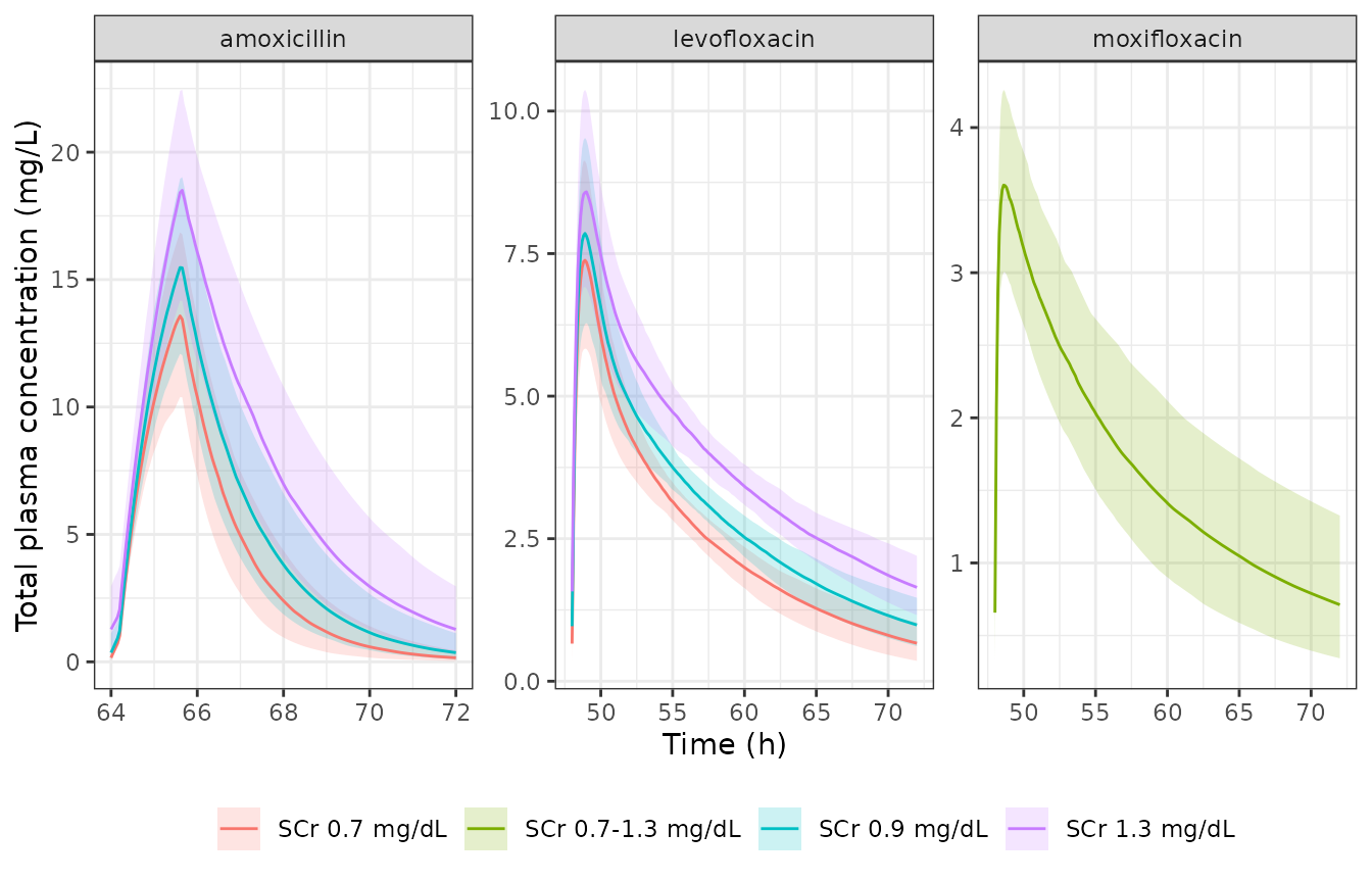
Simulated plasma concentrations on day 3 (median and 5th-95th percentiles) for adherent dosing, by drug and serum-creatinine subgroup.
PKNCA validation
Steady-state NCA over the last adherent dosing interval before the day-4 deviation: 64-72 h for amoxicillin and 48-72 h for the fluoroquinolones. Methods 4.3 states AUC0-24h = Dose / (CL/F) for the fluoroquinolones, so the reference AUC is the dose divided by the Supplementary Table S2 clearance. For amoxicillin the reference is F * Dose / CL from Table S1. Here F is the model’s total bioavailability at 1000 mg, F1 + (1 - F1) * DF = 0.150 + 0.850 * 1300 / 2300 = 0.631. The maintainers derived this reference value; the paper does not tabulate it.
ss <- sim |>
  filter(delay == 0) |>
  mutate(
    treatment = ifelse(is.na(creat), drug, paste0(drug, ", SCr ", creat)),
    start = ifelse(drug == "amoxicillin", 64, 48),
    end = 72
  ) |>
  filter(time >= start, time <= end, !is.na(Cc))

conc_obj <- PKNCAconc(ss, Cc ~ time | treatment + id)
dose_df <- ss |>
  distinct(treatment, id, drug, start) |>
  mutate(
    time = start,
    amt = case_when(drug == "amoxicillin" ~ 1000, drug == "levofloxacin" ~ 750, TRUE ~ 400)
  )
dose_obj <- PKNCAdose(dose_df, amt ~ time | treatment + id)
intervals <- ss |>
  distinct(treatment, start, end) |>
  mutate(cmax = TRUE, auclast = TRUE)
nca_res <- pk.nca(PKNCAdata(conc_obj, dose_obj, intervals = as.data.frame(intervals)))

f_amox <- expit(log(0.177)) + (1 - expit(log(0.177))) * 1300 / (1300 + 1000)
reference <- tibble(
  treatment = c(
    paste0("amoxicillin, SCr ", c(0.7, 0.9, 1.3)),
    paste0("levofloxacin, SCr ", c(0.7, 0.9, 1.3)),
    "moxifloxacin"
  ),
  auclast = c(f_amox * 1000 / c(20.1, 15.7, 10.8), 750 / c(14.9, 11, 9.7), 400 / 10.1)
)

cmp <- nlmixr2lib::ncaComparisonTable(
  simulated = nca_res,
  reference = reference,
  by = "treatment",
  params = "auclast",
  units = c(auclast = "mg*h/L"),
  tolerance_pct = 20
)
cmp |>
  dplyr::rename("Drug and subgroup" = treatment) |>
  knitr::kable(
    digits = 1,
    caption = paste(
      "Simulated median steady-state AUC over one dosing interval against",
      "(F *) Dose / CL from Supplementary Tables S1 and S2.",
      "* differs from the reference by more than 20%."
    )
)| NCA parameter | Drug and subgroup | Reference | Simulated | % diff |
|---|---|---|---|---|
| AUClast (mg*h/L) | amoxicillin, SCr 0.7 | 31.4 | 31.4 | +0.1% |
| AUClast (mg*h/L) | amoxicillin, SCr 0.9 | 40.2 | 39.9 | -0.8% |
| AUClast (mg*h/L) | amoxicillin, SCr 1.3 | 58.4 | 59.3 | +1.5% |
| AUClast (mg*h/L) | levofloxacin, SCr 0.7 | 50.3 | 60.6 | +20.4%* |
| AUClast (mg*h/L) | levofloxacin, SCr 0.9 | 68.2 | 72.8 | +6.7% |
| AUClast (mg*h/L) | levofloxacin, SCr 1.3 | 77.3 | 92.8 | +20.1%* |
| AUClast (mg*h/L) | moxifloxacin | 39.6 | 39.6 | +0.1% |
The amoxicillin and moxifloxacin AUCs agree with the supplement. The levofloxacin AUCs exceed the Table S2 references (by about 7-20%) because the printed clearance equation falls below Table S2 (see above).
auc_sim <- as.data.frame(nca_res) |>
  filter(PPTESTCD == "auclast") |>
  group_by(treatment) |>
  summarise(auc = median(PPORRES), .groups = "drop") |>
  inner_join(reference, by = "treatment") |>
  mutate(pct = 100 * (auc / auclast - 1))
# A mis-transcribed clearance, volume or bioavailability moves these
# medians by tens of percent.
stopifnot(all(abs(auc_sim$pct[!grepl("levofloxacin", auc_sim$treatment)]) < 10))
Replicating Table 1: probability of target attainment
The paper does not define the scoring window for a delayed dose. For amoxicillin, the maintainers found that Table 1 is reproduced when fT >= MIC is scored over the interval actually elapsed between the last on-time dose (64 h) and the delayed dose (72 + delay h), as a fraction of that interval’s length. A missed dose makes this a 16 h window. For the fluoroquinolones, fAUC0-24h is scored over the scheduled day-4 interval, 72-96 h. This reproduces the adherent and missed-dose columns; the delayed-dose columns match less well (see Assumptions and deviations). PTA is computed on the individual predictions, without residual error.
fu <- c(amoxicillin = 0.82, levofloxacin = 0.69, moxifloxacin = 0.52)
mic <- tribble(
  ~drug, ~setting, ~mic,
  "amoxicillin", "PHS", 0.064,
  "amoxicillin", "PLS", 1,
  "levofloxacin", "PHS", 0.064,
  "levofloxacin", "PLS", 1,
  "moxifloxacin", "PHS", 0.064,
  "moxifloxacin", "PLS", 0.25
)

# Amoxicillin: fraction of the elapsed interval [64, 72 + delay) with free
# concentration above the MIC.
pta_amox <- sim |>
  filter(drug == "amoxicillin", time >= 64, time < 72 + delay) |>
  inner_join(mic, by = "drug", relationship = "many-to-many") |>
  group_by(drug, creat, delay, setting, id) |>
  summarise(ft = mean(fu[["amoxicillin"]] * Cc > mic), .groups = "drop") |>
  group_by(drug, creat, delay, setting) |>
  summarise(pta = 100 * mean(ft >= 0.5), .groups = "drop")

# Fluoroquinolones: AUC over the scheduled day-4 interval, 72-96 h, with
# PKNCA's linear-up / log-down AUC calculation applied per virtual patient
# (the full pk.nca() object is too slow for 5,000 patient-scenarios).
pta_fq <- sim |>
  filter(drug != "amoxicillin", time >= 72, time <= 96, !is.na(Cc)) |>
  group_by(drug, creat, delay, id) |>
  summarise(auc = PKNCA::pk.calc.auc.last(conc = Cc, time = time - 72), .groups = "drop") |>
  inner_join(mic, by = "drug", relationship = "many-to-many") |>
  mutate(ratio = fu[drug] * auc / mic) |>
  group_by(drug, creat, delay, setting) |>
  summarise(pta = 100 * mean(ratio >= 33.8), .groups = "drop")

pta_sim <- bind_rows(pta_amox, pta_fq)
# Carral 2023 Table 1, transcribed. delay = dosing interval denotes the
# missed dose; `creat` NA is the pooled moxifloxacin group.
paper <- tribble(
  ~drug, ~creat, ~setting, ~delay, ~pta_paper,
  "amoxicillin", 0.7, "PHS", 0, 100, "amoxicillin", 0.7, "PHS", 6, 99, "amoxicillin", 0.7, "PHS", 7, 89, "amoxicillin", 0.7, "PHS", 8, 66,
  "amoxicillin", 0.9, "PHS", 0, 100, "amoxicillin", 0.9, "PHS", 6, 100, "amoxicillin", 0.9, "PHS", 7, 99, "amoxicillin", 0.9, "PHS", 8, 98,
  "amoxicillin", 1.3, "PHS", 0, 100, "amoxicillin", 1.3, "PHS", 6, 100, "amoxicillin", 1.3, "PHS", 7, 100, "amoxicillin", 1.3, "PHS", 8, 100,
  "amoxicillin", 0.7, "PLS", 0, 86, "amoxicillin", 0.7, "PLS", 1, 59, "amoxicillin", 0.7, "PLS", 2, 30, "amoxicillin", 0.7, "PLS", 3, 20,
  "amoxicillin", 0.7, "PLS", 4, 7, "amoxicillin", 0.7, "PLS", 5, 3, "amoxicillin", 0.7, "PLS", 8, 0,
  "amoxicillin", 0.9, "PLS", 0, 99, "amoxicillin", 0.9, "PLS", 1, 93, "amoxicillin", 0.9, "PLS", 2, 76, "amoxicillin", 0.9, "PLS", 3, 52,
  "amoxicillin", 0.9, "PLS", 4, 41, "amoxicillin", 0.9, "PLS", 5, 23, "amoxicillin", 0.9, "PLS", 8, 6,
  "amoxicillin", 1.3, "PLS", 0, 100, "amoxicillin", 1.3, "PLS", 1, 100, "amoxicillin", 1.3, "PLS", 2, 100, "amoxicillin", 1.3, "PLS", 3, 100,
  "amoxicillin", 1.3, "PLS", 4, 93, "amoxicillin", 1.3, "PLS", 5, 86, "amoxicillin", 1.3, "PLS", 8, 53,
  "levofloxacin", 0.7, "PHS", 0, 100, "levofloxacin", 0.7, "PHS", 12, 100, "levofloxacin", 0.7, "PHS", 24, 100,
  "levofloxacin", 0.9, "PHS", 0, 100, "levofloxacin", 0.9, "PHS", 12, 100, "levofloxacin", 0.9, "PHS", 24, 100,
  "levofloxacin", 1.3, "PHS", 0, 100, "levofloxacin", 1.3, "PHS", 12, 100, "levofloxacin", 1.3, "PHS", 24, 100,
  "levofloxacin", 0.7, "PLS", 0, 100, "levofloxacin", 0.7, "PLS", 6, 100, "levofloxacin", 0.7, "PLS", 8, 76,
  "levofloxacin", 0.7, "PLS", 12, 62, "levofloxacin", 0.7, "PLS", 14, 53, "levofloxacin", 0.7, "PLS", 24, 0,
  "levofloxacin", 0.9, "PLS", 0, 100, "levofloxacin", 0.9, "PLS", 6, 100, "levofloxacin", 0.9, "PLS", 8, 100,
  "levofloxacin", 0.9, "PLS", 12, 93, "levofloxacin", 0.9, "PLS", 14, 71, "levofloxacin", 0.9, "PLS", 24, 0,
  "levofloxacin", 1.3, "PLS", 0, 100, "levofloxacin", 1.3, "PLS", 6, 100, "levofloxacin", 1.3, "PLS", 8, 100,
  "levofloxacin", 1.3, "PLS", 12, 100, "levofloxacin", 1.3, "PLS", 14, 100, "levofloxacin", 1.3, "PLS", 24, 0,
  "moxifloxacin", NA, "PHS", 0, 100, "moxifloxacin", NA, "PHS", 12, 100, "moxifloxacin", NA, "PHS", 24, 100,
  "moxifloxacin", NA, "PLS", 0, 100, "moxifloxacin", NA, "PLS", 1, 100, "moxifloxacin", NA, "PLS", 4, 100,
  "moxifloxacin", NA, "PLS", 6, 100, "moxifloxacin", NA, "PLS", 12, 100, "moxifloxacin", NA, "PLS", 14, 100,
  "moxifloxacin", NA, "PLS", 24, 0
)

table1 <- paper |>
  left_join(pta_sim, by = c("drug", "creat", "setting", "delay")) |>
  mutate(
    crcl = case_when(creat == 0.7 ~ "131", creat == 0.9 ~ "100", creat == 1.3 ~ "70", TRUE ~ "70-131"),
    scenario = case_when(
      delay == 0 ~ "adherent",
      (drug == "amoxicillin" & delay == 8) | delay == 24 ~ "missed dose",
      TRUE ~ paste0("delayed ", delay, " h")
    )
  )

table1 |>
  select(drug, setting, crcl, scenario, pta_paper, pta) |>
  rename(
    "Drug" = drug,
    "MIC setting" = setting,
    "CLcr (mL/min)" = crcl,
    "Scenario" = scenario,
    "PTA, Table 1 (%)" = pta_paper,
    "PTA, simulated (%)" = pta
  ) |>
knitr::kable(digits = 0, caption = "Replicates Table 1 of Carral 2023: % PTA by drug, MIC setting, renal subgroup and adherence scenario.")| Drug | MIC setting | CLcr (mL/min) | Scenario | PTA, Table 1 (%) | PTA, simulated (%) |
|---|---|---|---|---|---|
| amoxicillin | PHS | 131 | adherent | 100 | 100 |
| amoxicillin | PHS | 131 | delayed 6 h | 99 | 95 |
| amoxicillin | PHS | 131 | delayed 7 h | 89 | 88 |
| amoxicillin | PHS | 131 | missed dose | 66 | 79 |
| amoxicillin | PHS | 100 | adherent | 100 | 100 |
| amoxicillin | PHS | 100 | delayed 6 h | 100 | 98 |
| amoxicillin | PHS | 100 | delayed 7 h | 99 | 98 |
| amoxicillin | PHS | 100 | missed dose | 98 | 96 |
| amoxicillin | PHS | 70 | adherent | 100 | 100 |
| amoxicillin | PHS | 70 | delayed 6 h | 100 | 100 |
| amoxicillin | PHS | 70 | delayed 7 h | 100 | 100 |
| amoxicillin | PHS | 70 | missed dose | 100 | 100 |
| amoxicillin | PLS | 131 | adherent | 86 | 83 |
| amoxicillin | PLS | 131 | delayed 1 h | 59 | 62 |
| amoxicillin | PLS | 131 | delayed 2 h | 30 | 38 |
| amoxicillin | PLS | 131 | delayed 3 h | 20 | 18 |
| amoxicillin | PLS | 131 | delayed 4 h | 7 | 6 |
| amoxicillin | PLS | 131 | delayed 5 h | 3 | 1 |
| amoxicillin | PLS | 131 | missed dose | 0 | 0 |
| amoxicillin | PLS | 100 | adherent | 99 | 98 |
| amoxicillin | PLS | 100 | delayed 1 h | 93 | 94 |
| amoxicillin | PLS | 100 | delayed 2 h | 76 | 80 |
| amoxicillin | PLS | 100 | delayed 3 h | 52 | 60 |
| amoxicillin | PLS | 100 | delayed 4 h | 41 | 41 |
| amoxicillin | PLS | 100 | delayed 5 h | 23 | 26 |
| amoxicillin | PLS | 100 | missed dose | 6 | 4 |
| amoxicillin | PLS | 70 | adherent | 100 | 100 |
| amoxicillin | PLS | 70 | delayed 1 h | 100 | 100 |
| amoxicillin | PLS | 70 | delayed 2 h | 100 | 99 |
| amoxicillin | PLS | 70 | delayed 3 h | 100 | 96 |
| amoxicillin | PLS | 70 | delayed 4 h | 93 | 92 |
| amoxicillin | PLS | 70 | delayed 5 h | 86 | 85 |
| amoxicillin | PLS | 70 | missed dose | 53 | 52 |
| levofloxacin | PHS | 131 | adherent | 100 | 100 |
| levofloxacin | PHS | 131 | delayed 12 h | 100 | 100 |
| levofloxacin | PHS | 131 | missed dose | 100 | 92 |
| levofloxacin | PHS | 100 | adherent | 100 | 100 |
| levofloxacin | PHS | 100 | delayed 12 h | 100 | 100 |
| levofloxacin | PHS | 100 | missed dose | 100 | 99 |
| levofloxacin | PHS | 70 | adherent | 100 | 100 |
| levofloxacin | PHS | 70 | delayed 12 h | 100 | 100 |
| levofloxacin | PHS | 70 | missed dose | 100 | 100 |
| levofloxacin | PLS | 131 | adherent | 100 | 100 |
| levofloxacin | PLS | 131 | delayed 6 h | 100 | 100 |
| levofloxacin | PLS | 131 | delayed 8 h | 76 | 97 |
| levofloxacin | PLS | 131 | delayed 12 h | 62 | 40 |
| levofloxacin | PLS | 131 | delayed 14 h | 53 | 4 |
| levofloxacin | PLS | 131 | missed dose | 0 | 0 |
| levofloxacin | PLS | 100 | adherent | 100 | 100 |
| levofloxacin | PLS | 100 | delayed 6 h | 100 | 100 |
| levofloxacin | PLS | 100 | delayed 8 h | 100 | 100 |
| levofloxacin | PLS | 100 | delayed 12 h | 93 | 100 |
| levofloxacin | PLS | 100 | delayed 14 h | 71 | 90 |
| levofloxacin | PLS | 100 | missed dose | 0 | 0 |
| levofloxacin | PLS | 70 | adherent | 100 | 100 |
| levofloxacin | PLS | 70 | delayed 6 h | 100 | 100 |
| levofloxacin | PLS | 70 | delayed 8 h | 100 | 100 |
| levofloxacin | PLS | 70 | delayed 12 h | 100 | 100 |
| levofloxacin | PLS | 70 | delayed 14 h | 100 | 100 |
| levofloxacin | PLS | 70 | missed dose | 0 | 0 |
| moxifloxacin | PHS | 70-131 | adherent | 100 | 100 |
| moxifloxacin | PHS | 70-131 | delayed 12 h | 100 | 100 |
| moxifloxacin | PHS | 70-131 | missed dose | 100 | 94 |
| moxifloxacin | PLS | 70-131 | adherent | 100 | 100 |
| moxifloxacin | PLS | 70-131 | delayed 1 h | 100 | 100 |
| moxifloxacin | PLS | 70-131 | delayed 4 h | 100 | 100 |
| moxifloxacin | PLS | 70-131 | delayed 6 h | 100 | 100 |
| moxifloxacin | PLS | 70-131 | delayed 12 h | 100 | 100 |
| moxifloxacin | PLS | 70-131 | delayed 14 h | 100 | 100 |
| moxifloxacin | PLS | 70-131 | missed dose | 0 | 12 |
amox_pls <- table1 |> filter(drug == "amoxicillin", setting == "PLS")
adherent <- table1 |> filter(delay == 0)
missed_fq_pls <- table1 |> filter(drug != "amoxicillin", setting == "PLS", delay == 24)
stopifnot(
  # The amoxicillin PLS rows carry the paper's gradient over delay and renal
  # function; a wrong clearance, volume or absorption split shifts the whole
  # curve. Centre and robust envelope only (see the cohort note above).
  abs(median(amox_pls$pta - amox_pls$pta_paper)) < 10,
  quantile(abs(amox_pls$pta - amox_pls$pta_paper), 0.9) < 20,
  # Adherent dosing meets the target in (nearly) every group but amoxicillin
  # at CLcr 131 mL/min with MIC 1 mg/L.
  all(abs(adherent$pta - adherent$pta_paper) < 15),
  # A missed fluoroquinolone dose fails the low-susceptibility target.
  all(missed_fq_pls$pta < 25)
)
Replicating Figures 1 and 2: relative forgiveness
Relative forgiveness is the odds ratio of the PTA under imperfect adherence to the PTA under perfect adherence (Methods 4.4). A PTA of 0% or 100% has infinite odds, so both the simulated and the Table 1 PTAs are clamped to [0.5, 99.5]%. This gives RF = 1 when both scenarios reach 100%. The paper does not say how it treated these boundary values.
odds <- function(p) {
  p <- pmin(pmax(p / 100, 0.005), 0.995)
  p / (1 - p)
}
rf <- table1 |>
  filter(setting == "PLS") |>
  group_by(drug, crcl) |>
  mutate(
    rf_sim = odds(pta) / odds(pta[delay == 0]),
    rf_paper = odds(pta_paper) / odds(pta_paper[delay == 0])
  ) |>
  ungroup() |>
  filter(delay > 0) |>
  mutate(
    scenario = factor(scenario, levels = unique(scenario[order(delay)])),
    crcl = factor(crcl, levels = c("131", "100", "70", "70-131"))
  )

ggplot(rf, aes(scenario, rf_sim, fill = crcl)) +
  geom_col(position = position_dodge(width = 0.8), width = 0.7) +
  geom_point(aes(y = rf_paper, group = crcl), position = position_dodge(width = 0.8), shape = 21, colour = "black", fill = "white") +
  facet_wrap(~drug, scales = "free_x") +
  coord_cartesian(ylim = c(0, 1.1)) +
  labs(x = NULL, y = "Relative forgiveness", fill = "CLcr (mL/min)") +
  theme_bw() +
  theme(axis.text.x = element_text(angle = 45, hjust = 1), legend.position = "bottom")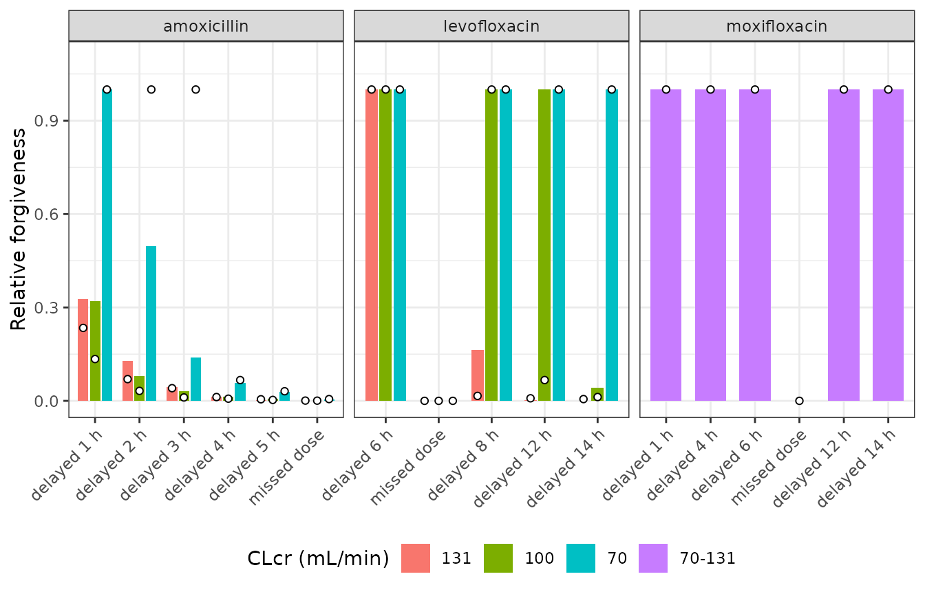
Replicates Figures 1 and 2 of Carral 2023: relative forgiveness of each drug in the low-susceptibility (PLS) setting, from the simulated PTA (bars) and from the Table 1 PTA (points).
Figure 3 of the paper compares the fluoroquinolones with amoxicillin (RF(B:A), Methods 4.5). Its values reach about 1900 at CLcr 130 mL/min, which depends on how a 0% amoxicillin PTA was handled in the odds. The paper does not state this, so Figure 3 is not reproduced quantitatively. Qualitatively, the simulated PTAs above give RF(B:A) > 1 that grows with the delay and with creatinine clearance, as in the figure.
Assumptions and deviations
-
Simulation-only parameter values. All three
appendices are NONMEM
ONLYSIMcontrol streams. Their$THETA/$OMEGA/$SIGMAvalues are the values the authors simulated from; this paper estimated none of them. The levofloxacin and moxifloxacin structures come from Preston et al. (1998) and Grosjean and Urien (2012). The omega values are the authors’ choices (“the variability was also set to a typical range”, Discussion). -
Virtual covariates as data columns. Each stream
generates age, weight, ideal body weight or lean body mass per virtual
patient with an ETA (for example
SIMAGE = 45*EXP(ETA(6))). The packaged models take these as data columns (AGE,WT,IBW,LBM) so they can be used with real patients. The vignette reproduces the streams’ draws in the cohort, so the simulated population is the same. -
Serum creatinine as a covariate. The renal
subgroups differ only in serum creatinine (0.7, 0.9, 1.3 mg/dL). The
amoxicillin stream reads it as
Cr. The levofloxacin stream as printed hard-codes 0.9 mg/dL (the middle subgroup), and its THETA(1) = 0.7 ‘Blood creatine mean value’ is not used in the printed$PK. Both models useCREATin the male Cockcroft-Gault equation. -
First amoxicillin omega. The
$OMEGAline is printed as; 004 0.036 0.01 0.04 0.001 0.025. The second to sixth values fit the six ETAs in order (KA, CL, V, KD, weight, age). The weight and age values reproduce the Table S1 CLcr spread (+/- 10, 8 and 6 mL/min). The garbled first entry is read as 0.04, the 20% CV that Methods 4.2 states for the PK parameters. - Amoxicillin V/F spread. With omega^2 = 0.01 on V/F and 0.001 on weight, the simulated V/F has a CV of about 10.5%. Table S1 lists 23.3 +/- 3.9 L (17%). The printed omega is kept.
-
Amoxicillin residual error.
W = IPRE + .001; Y = F + W*EPS(1)with$SIGMA 0.4is a combined error whose standard deviations add (combined1()), with proportional SD sqrt(0.4) = 0.63 and additive SD 0.001 * sqrt(0.4) mg/L. The PTA analyses use the individual predictions, where residual error plays no part. -
Moxifloxacin Q/F. Appendix C prints
TVQ=THETA(4)* ((SIMLBM/(60)**0.75)with an unbalanced parenthesis. A literal Fortran reading, SIMLBM / 60^0.75, would make Q/F 2.8 times larger. The model uses (LBM/60)^0.75, the same form as CL/F on the line above. - Levofloxacin clearance vs Table S2. The printed regression gives clearances 7-18% below Table S2. Table S2 is not linear in CLcr, and its 14.9 L/h at CLcr 131 mL/min would give an adherent fAUC/MIC of 0.69 * 750 / 14.9 = 34.7, at the 33.8 threshold, so about half the patients would miss the target. Table 1 reports 100%. The printed equation gives 42 and reproduces Table 1.
- Scoring windows. The paper does not define how fT >= MIC and fAUC0-24h were scored around a delayed dose. The windows used here (see the Table 1 section) were chosen by the maintainers because they reproduce Table 1. With them, the amoxicillin rows and the adherent and missed-dose fluoroquinolone rows agree with the paper. The levofloxacin delayed-dose rows at CLcr 131 mL/min fall faster than in the paper (8 h: about 97% vs 76%; 12 h: about 40% vs 62%; 14 h: under 10% vs 53%). The model’s very small clearance variability (omega^2 = 0.001) makes the simulated PTA close to a step function of the delay. The paper’s gentler decline cannot come from the printed omegas under either window the maintainers tried. The moxifloxacin missed-dose PTA in the low-susceptibility setting comes out at about 10-15% rather than 0%. The missed-dose PTA in the high-susceptibility setting comes out at about 90-95% at CLcr 131 mL/min, where the paper reports 100%.
- Cohort size. 200 virtual patients per drug, renal subgroup and scenario, against the paper’s 10,000.