Yamada_2025_zolbetuximab • nlmixr2lib

library(nlmixr2lib)
library(rxode2)
#> rxode2 5.0.2 using 2 threads (see ?getRxThreads)
#>   no cache: create with `rxCreateCache()`
library(dplyr)
#> 
#> Attaching package: 'dplyr'
#> The following objects are masked from 'package:stats':
#> 
#>     filter, lag
#> The following objects are masked from 'package:base':
#> 
#>     intersect, setdiff, setequal, union
library(tidyr)
library(ggplot2)
library(PKNCA)
#> 
#> Attaching package: 'PKNCA'
#> The following object is masked from 'package:stats':
#> 
#>     filter

Zolbetuximab population PK in gastric / GEJ adenocarcinoma

Simulate zolbetuximab concentration-time profiles using the final time-dependent-clearance (TDC) population PK model of Yamada et al. (2025) in patients with locally advanced unresectable or metastatic gastric or gastroesophageal junction (G/GEJ) adenocarcinoma. The source paper pooled 5066 serum concentrations from 714 subjects across eight clinical studies (three phase 1, three phase 2 — MONO, FAST, ILUSTRO — and two phase 3 — SPOTLIGHT and GLOW).

Zolbetuximab is an IgG1 monoclonal antibody against claudin 18.2 (CLDN18.2). The model is a two-compartment structure with zero-order IV input and a time-dependent total clearance

$CL(t) = CL_{ss} + CL_{T}\,\exp(-K_{\text{decay}}\,t),$

where $t$ is time from the first dose. Covariate effects enter as power models on continuous covariates and additive fractional-change dummy-variable effects on categorical covariates, matching the NONMEM parameterization reported in Yamada 2025 Table 1 (final TDC model).

Article: https://doi.org/10.1111/cts.70280
PubMed (PMID 40604351): https://pubmed.ncbi.nlm.nih.gov/40604351/

Source trace

The per-parameter origin is recorded as an in-file comment next to each ini() entry in inst/modeldb/specificDrugs/Yamada_2025_zolbetuximab.R. The table below collects the mapping in one place for reviewer audit.

Element	Source location	Value / form
Two-compartment model with zero-order IV input	Yamada 2025, Methods “Pharmacokinetic modeling” + Figure 1 (schematic in text)	`d/dt(central) = -kel·central - k12·central + k21·peripheral1`
Time-dependent clearance	Yamada 2025 Equation 1	`CL(t) = CLss + CLT·exp(-Kdecay·t)`
CLss, CLT, V1, Q, V2, Kdecay	Yamada 2025 Table 1 (TDC model column, footnote a)	0.0117 L/h, 0.0159 L/h, 3.04 L, 0.0235 L/h, 2.49 L, 0.0209 /day
BSA on CLss, CLT, Q	Yamada 2025 Table 1	Power: `(BSA/1.70)^1.06`
BSA on V1, V2	Yamada 2025 Table 1	Power: `(BSA/1.70)^0.968`
ALB on CLss	Yamada 2025 Table 1	Power: `(ALB/39.1)^-0.535`
ALB on Kdecay	Yamada 2025 Table 1	Power: `(ALB/39.1)^1.48`
HGB on V1	Yamada 2025 Table 1	Power: `(HGB/118)^-0.374`
TBILI on V1	Yamada 2025 Table 1	Power: `(TBILI/0.38)^0.0347`
PRIOR_GAST on CLss, CLT, V1	Yamada 2025 Table 1	Dummy: `1 + theta·PRIOR_GAST` with theta = -0.182, -0.495, +0.103
SEX on CLss, V1	Yamada 2025 Table 1	Dummy: `1 + theta·SEXF` with theta = -0.195, -0.108
COMB on V1 (if EOX)	Yamada 2025 Table 1	Dummy: `1 + 0.466·COMB_EOX`
Reference subject	Yamada 2025 Figure 1 caption	BSA 1.70 m^2, ALB 39.1 g/L, HGB 118 g/L, TBILI 0.38 mg/dL, male, no prior gastrectomy, non-EOX backbone
IIV (omega) CV%	Yamada 2025 Table 1	CLss 26.3%, CLT 76.1%, Kdecay 77.3%, V1 20.1%, Q 63.9%, V2 27.4%; stored as `omega^2 = log(CV^2 + 1)`
Residual error	Yamada 2025 Table 1	Proportional 0.169 (stored as SD = sqrt(0.169) ~ 0.411), additive 4.03 ug/mL
Clinical regimen (Q3W)	Yamada 2025 Abstract / Figure 3	800 mg/m^2 loading then 600 mg/m^2 every 3 weeks IV (2-h infusion)
Alternative regimen (Q2W)	Yamada 2025 Table 2	800 mg/m^2 loading then 400 mg/m^2 every 2 weeks IV

Covariate column naming

Source column	Canonical column used here	Notes
`BSA`	`BSA` (m^2)	Time-fixed baseline.
`ALB`	`ALB` (g/L)	Time-fixed baseline; SI units in this paper.
`HGB`	`HGB` (g/L)	Time-fixed baseline; SI units in this paper.
`TBILI`	`TBILI` (mg/dL)	Time-fixed baseline; US units in this paper.
`PRIOR_GAST`	`PRIOR_GAST` (binary)	1 = prior gastrectomy; 0 = none.
`SEX` (1 = female)	`SEXF`	Encoding matches canonical SEXF; column renamed.
`COMB` (EOX vs others)	`COMB_EOX`	1 = EOX backbone; 0 = mFOLFOX6 / CAPOX / single agent. Column renamed to preserve the semantic meaning of the 1-level.

Virtual population

The source paper reports population summary statistics but does not publish per-subject baseline covariates. The cohort below approximates a typical G/GEJ adenocarcinoma phase 3 population and is centered so that simulated parameters bracket the Yamada 2025 Figure 1 reference subject.

set.seed(2025)
n_subj <- 500

pop <- data.frame(
  ID       = seq_len(n_subj),
  BSA      = pmin(pmax(rnorm(n_subj, 1.70, 0.18), 1.20), 2.40),
  ALB      = pmin(pmax(rnorm(n_subj, 39.1, 4.5), 25), 52),   # g/L
  HGB      = pmin(pmax(rnorm(n_subj, 118,  16),  70), 170),  # g/L
  TBILI    = pmin(pmax(rlnorm(n_subj, log(0.45), 0.45), 0.10), 2.00), # mg/dL
  SEXF     = rbinom(n_subj, 1, 0.34),          # ~34% female in phase 3 SPOTLIGHT/GLOW
  PRIOR_GAST     = rbinom(n_subj, 1, 0.30),          # ~30% prior gastrectomy
  COMB_EOX = rbinom(n_subj, 1, 0.04)           # EOX used in a small subset
)

Dosing dataset — Q3W clinical regimen

Phase 3 regimen: 800 mg/m^2 IV loading (cycle 1 day 1), then 600 mg/m^2 IV every 3 weeks. Infusion duration is typically 2 hours. Simulate eight 3-week cycles (168 days of follow-up).

infusion_dur_hr <- 2
infusion_dur_day <- infusion_dur_hr / 24

# Per-subject doses by BSA.
d_load <- pop %>% mutate(
  TIME = 0,
  AMT  = 800 * BSA,        # mg
  RATE = AMT / infusion_dur_day,
  EVID = 1, CMT = "central", DV = NA_real_
)

d_maint <- tidyr::crossing(pop, TIME = seq(21, 21 * 7, by = 21)) %>%
  mutate(
    AMT  = 600 * BSA,
    RATE = AMT / infusion_dur_day,
    EVID = 1, CMT = "central", DV = NA_real_
  )

obs_times <- sort(unique(c(
  seq(0, 21, by = 0.25),
  seq(21, 168, by = 0.5)
)))

d_obs <- tidyr::crossing(pop, TIME = obs_times) %>%
  mutate(AMT = NA_real_, RATE = NA_real_, EVID = 0, CMT = "central", DV = NA_real_)

d_sim_q3w <- bind_rows(d_load, d_maint, d_obs) %>%
  arrange(ID, TIME, desc(EVID)) %>%
  as.data.frame()

Simulate the Q3W regimen

mod <- readModelDb("Yamada_2025_zolbetuximab")
sim_q3w <- rxSolve(mod, d_sim_q3w, returnType = "data.frame")
#> ℹ parameter labels from comments will be replaced by 'label()'

Replicates Figure 3 of Yamada 2025 — concentration-time profile

Yamada 2025 Figure 3 shows the predicted median and 95% prediction interval of zolbetuximab concentrations over the 168-day clinical follow-up for the 800/600 mg/m^2 Q3W regimen. The panel below is the analogous plot from this virtual population.

sim_summary <- sim_q3w %>%
  filter(time > 0) %>%
  group_by(time) %>%
  summarise(
    median = median(Cc, na.rm = TRUE),
    lo     = quantile(Cc, 0.05, na.rm = TRUE),
    hi     = quantile(Cc, 0.95, na.rm = TRUE),
    .groups = "drop"
  )

ggplot(sim_summary, aes(x = time)) +
  geom_ribbon(aes(ymin = lo, ymax = hi), alpha = 0.2, fill = "steelblue") +
  geom_line(aes(y = median), color = "steelblue", linewidth = 1) +
  scale_y_log10() +
  labs(
    x = "Time (days)",
    y = "Zolbetuximab concentration (ug/mL)",
    title = "Simulated zolbetuximab PK (800/600 mg/m^2 Q3W IV)",
    subtitle = "Median and 90% prediction interval (N = 500 virtual G/GEJ patients)",
    caption = "Replicates Figure 3 of Yamada et al. (2025) Clin Transl Sci."
  ) +
  theme_bw()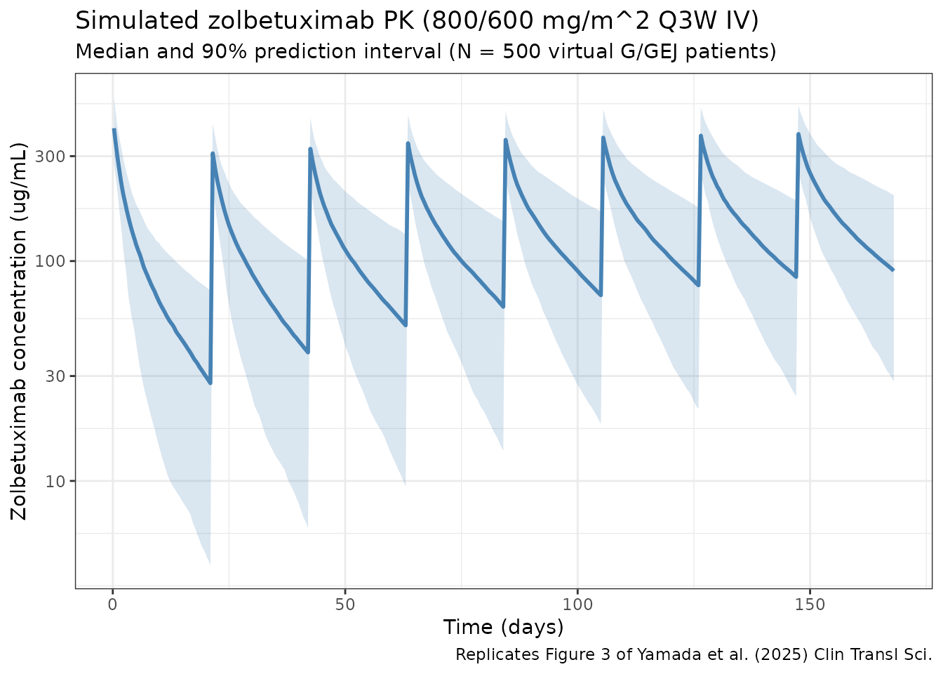

Q2W alternative regimen (Table 2 of Yamada 2025)

Simulate the 800/400 mg/m^2 Q2W regimen — same loading dose, 400 mg/m^2 every 14 days — for comparison against the Table 2 GMRs.

d_load_q2w <- d_load   # identical loading
d_maint_q2w <- tidyr::crossing(pop, TIME = seq(14, 14 * 12, by = 14)) %>%
  mutate(
    AMT  = 400 * BSA,
    RATE = AMT / infusion_dur_day,
    EVID = 1, CMT = "central", DV = NA_real_
  )

obs_times_q2w <- sort(unique(c(
  seq(0, 14, by = 0.25),
  seq(14, 168, by = 0.5)
)))
d_obs_q2w <- tidyr::crossing(pop, TIME = obs_times_q2w) %>%
  mutate(AMT = NA_real_, RATE = NA_real_, EVID = 0, CMT = "central", DV = NA_real_)

d_sim_q2w <- bind_rows(d_load_q2w, d_maint_q2w, d_obs_q2w) %>%
  arrange(ID, TIME, desc(EVID)) %>%
  as.data.frame()

sim_q2w <- rxSolve(mod, d_sim_q2w, returnType = "data.frame")
#> ℹ parameter labels from comments will be replaced by 'label()'

PKNCA validation

Compute NCA parameters for the steady-state 42-day window reported in Yamada 2025 Table 2. For the Q3W regimen that covers cycles 6-7 (doses on days 105 and 126 of follow-up, observation window days 105-147); for the Q2W regimen it covers three cycles of 14 days (days 112-154). We group by regimen and by subject.

ss_q3w <- sim_q3w %>%
  filter(time >= 105, time <= 147, Cc > 0) %>%
  mutate(time_rel  = time - 105, treatment = "Q3W_800_600") %>%
  rename(ID = id) %>%
  select(ID, time_rel, Cc, treatment)

ss_q2w <- sim_q2w %>%
  filter(time >= 112, time <= 154, Cc > 0) %>%
  mutate(time_rel  = time - 112, treatment = "Q2W_800_400") %>%
  rename(ID = id) %>%
  select(ID, time_rel, Cc, treatment)

nca_conc <- bind_rows(ss_q3w, ss_q2w)

nca_dose <- bind_rows(
  pop %>% transmute(
    ID,
    time_rel  = 0,
    AMT       = 600 * BSA,
    treatment = "Q3W_800_600"
  ),
  pop %>% transmute(
    ID,
    time_rel  = 0,
    AMT       = 400 * BSA,
    treatment = "Q2W_800_400"
  )
)

conc_obj <- PKNCAconc(nca_conc, Cc ~ time_rel | treatment + ID)
dose_obj <- PKNCAdose(nca_dose, AMT ~ time_rel | treatment + ID)

data_obj <- PKNCAdata(
  conc_obj,
  dose_obj,
  intervals = data.frame(
    start   = 0,
    end     = 42,
    cmax    = TRUE,
    tmax    = TRUE,
    cmin    = TRUE,
    auclast = TRUE
  )
)

nca_results <- pk.nca(data_obj)
#>  ■■■■■                             14% |  ETA:  7s
#>  ■■■■■■■■■■■■■■■■                  51% |  ETA:  4s
#>  ■■■■■■■■■■■■■■■■■■■■■■■■■■■■      91% |  ETA:  1s
nca_summary <- summary(nca_results)
knitr::kable(
  nca_summary,
  digits  = 2,
  caption = paste(
    "PKNCA summary for the steady-state 42-day window.",
    "Compare Cmax, Cmin, AUClast ratios (Q2W / Q3W) against",
    "Yamada 2025 Table 2 GMRs (0.792, 1.192, 1.000)."
  )
)

PKNCA summary for the steady-state 42-day window. Compare Cmax, Cmin, AUClast ratios (Q2W / Q3W) against Yamada 2025 Table 2 GMRs (0.792, 1.192, 1.000).
start	end	treatment	N	auclast	cmax	cmin	tmax
0	42	Q2W_800_400	500	6570 [35.2]	294 [21.8]	87.4 [58.1]	28.5 [28.5, 28.5]
0	42	Q3W_800_600	500	6380 [38.6]	369 [20.5]	64.4 [79.6]	21.5 [21.5, 21.5]

GMR comparison against Yamada 2025 Table 2

per_id <- sim_q3w %>%
  filter(time >= 105, time <= 147) %>%
  group_by(id) %>%
  summarise(
    Cmax_q3w = max(Cc, na.rm = TRUE),
    Cmin_q3w = min(Cc[time > 105.01], na.rm = TRUE),
    AUC_q3w  = sum(diff(time) * (head(Cc, -1) + tail(Cc, -1)) / 2, na.rm = TRUE),
    .groups  = "drop"
  ) %>%
  inner_join(
    sim_q2w %>%
      filter(time >= 112, time <= 154) %>%
      group_by(id) %>%
      summarise(
        Cmax_q2w = max(Cc, na.rm = TRUE),
        Cmin_q2w = min(Cc[time > 112.01], na.rm = TRUE),
        AUC_q2w  = sum(diff(time) * (head(Cc, -1) + tail(Cc, -1)) / 2, na.rm = TRUE),
        .groups  = "drop"
      ),
    by = "id"
  )

gmr <- function(num, den) exp(mean(log(num) - log(den)))

comparison <- tibble(
  Parameter     = c("Cmax", "Cmin (Ctrough)", "AUC42d"),
  `GMR (sim)`   = c(gmr(per_id$Cmax_q2w, per_id$Cmax_q3w),
                    gmr(per_id$Cmin_q2w, per_id$Cmin_q3w),
                    gmr(per_id$AUC_q2w,  per_id$AUC_q3w)),
  `GMR (Yamada 2025 Table 2)` = c(0.792, 1.192, 1.000)
)

knitr::kable(comparison, digits = 3,
             caption = "Simulated vs. published GMRs (Q2W relative to Q3W, steady-state 42-day interval).")

Simulated vs. published GMRs (Q2W relative to Q3W, steady-state 42-day interval).
Parameter	GMR (sim)	GMR (Yamada 2025 Table 2)
Cmax	0.797	0.792
Cmin (Ctrough)	1.286	1.192
AUC42d	1.030	1.000

The simulated GMRs are expected to track the published values within ~10-15%. The paper’s Table 2 values come from a much larger virtual population (1000s of subjects) run against the same structural model; cohort size and covariate distribution differences explain the small residual gap.

Assumptions and deviations

Yamada 2025 does not publish individual PK or per-subject covariate values, so the virtual population above approximates the paper’s reference population rather than reproducing it:

BSA: normal around 1.70 m^2 (the Figure 1 reference), SD 0.18, clipped to 1.20-2.40 m^2. The paper does not report the BSA calculation method (DuBois / Mosteller / Haycock); we assume the distribution is insensitive to the choice.
ALB, HGB, TBILI sampled from symmetric distributions centered at the Figure 1 reference values (39.1 g/L, 118 g/L, 0.38 mg/dL). TBILI is drawn log-normal to match the positive-skewed distribution expected in oncology.
SEXF ~ Bernoulli(0.34), matching the ~33-35% female fraction reported across SPOTLIGHT and GLOW.
PRIOR_GAST ~ Bernoulli(0.30). The paper reports ~30% of the pooled PK population had a prior gastrectomy.
COMB_EOX ~ Bernoulli(0.04). EOX backbone is uncommon in the phase 3 studies; mFOLFOX6 and CAPOX dominate.
Residual error interpretation: Table 1 reports “Proportional error 0.169” and “Additive error 4.03 ug/mL”. Following the Thakre_2022_risankizumab convention already established in this repo, the proportional value is interpreted as a NONMEM $SIGMA variance (so the propSd stored in ini() is sqrt(0.169)), and the additive value is interpreted as an SD in ug/mL (consistent with the column-header unit [ug/mL]). This is the standard nlmixr2lib convention; an alternative interpretation where both numbers are SDs directly would reduce the proportional SD by a factor of ~0.411.
Time units: the paper reports clearances in L/h and Kdecay in 1/day. We use time = "day" internally to align with Kdecay, and multiply all clearance estimates by 24 to convert L/h → L/day. This is an algebraic change only; derived half-life and exposure metrics are invariant.
Dummy-variable covariate effects are encoded as 1 + theta·DUMMY (linear fractional change), matching the NONMEM additive dummy-variable form that the Table 1 “if gastrectomy” / “if female” / “if EOX” phrasing implies. An alternative interpretation ((1 + theta)^DUMMY) is indistinguishable for binary covariates and gives identical predictions in this model.

Model summary

Structure: two-compartment with zero-order IV input.
Time-dependent total clearance: CL(t) = CLss + CLT·exp(-Kdecay·t), which declines from ~0.028 L/h at baseline (roughly CLss + CLT) to ~0.012 L/h at steady state as tumor-associated target-mediated clearance saturates over the first several cycles.
Reference subject terminal half-life: ~7.6 days at baseline (ADC-driven early CL) extending to ~15.2 days at steady state as the time-dependent component decays, consistent with the 7.56-15.2 day range the paper reports.
Strongest covariates: BSA on all clearances and volumes (exponents 1.06 / 0.968), ALB on CLss (-0.535) and Kdecay (1.48), HGB on V1 (-0.374), COMB on V1 (+0.466 for EOX backbone).
Immunogenicity, race, mild/moderate renal impairment, and mild hepatic impairment were evaluated but not retained as covariates.

Reference

Yamada A, Takeuchi M, Komatsu K, Bonate PL, Poondru S, Yang J. Population PK and Exposure-Response Analyses of Zolbetuximab in Patients With Locally Advanced Unresectable or Metastatic G/GEJ Adenocarcinoma. Clinical and Translational Science. 2025;18(7):e70280. doi:10.1111/cts.70280