Tazobactam (Williamson 2026)
Source:vignettes/articles/Williamson_2026_tazobactam.Rmd
Williamson_2026_tazobactam.RmdModel and source
#> ℹ parameter labels from comments will be replaced by 'label()'Citation: Williamson R, Zurawska M, Valadez A, Harlan E, Scheetz MH, Neely MN, Yarnold PR, Kang M, Donnelly HK, Martinez F, Korth E, Medernach RL, Nozick SH, Hauser AR, Ozer EA, Diaz E, Misharin AV, Wunderink RG, Rhodes NJ. Critical threshold target attainment rates for tazobactam combined with piperacillin among patients admitted to the ICU with hospital-acquired pneumonia. Antimicrob Agents Chemother. 2026;70(2):e01766-25. doi:10.1128/aac.01766-25.
Description: One-compartment population PK model for tazobactam (given with piperacillin) in critically ill adults with hospital-acquired pneumonia (Williamson 2026). Total clearance is a piecewise sum of four arms: a creatinine-clearance-scaled renal arm and a non-renal arm, both switched off whenever renal replacement is running, plus an effluent-flow-scaled continuous-renal-replacement arm and a literature-fixed intermittent- hemodialysis arm. Unbound concentration uses a fixed 70% unbound fraction.
Article: https://doi.org/10.1128/aac.01766-25
PubMed Central: https://www.ncbi.nlm.nih.gov/pmc/articles/PMC12888870/
Companion piperacillin model from the same cohort:
readModelDb("Zurawska_2026_piperacillin")(https://doi.org/10.1128/aac.01760-25)
Williamson and colleagues developed a population PK model of the beta-lactamase inhibitor tazobactam in critically ill adults with hospital-acquired pneumonia, including patients on continuous renal replacement therapy (CRRT), and used it to ask how often standard tazobactam regimens keep the unbound concentration above 1, 2 or 4 mg/L for the whole of the second day of treatment (100% fT > threshold between 24 and 48 h).
Clearance has the same four-arm piecewise structure as the companion
piperacillin model: a renal arm scaled by Cockcroft-Gault creatinine
clearance and a non-renal arm are summed, that sum is switched
off whenever either renal-replacement modality is
running, and an effluent-flow-scaled CRRT arm and a literature-fixed
intermittent-hemodialysis arm are added on top. The model also carries
the paper’s fixed 70% unbound fraction as the output
Cu.
Population
35 critically ill adults contributed 162 plasma samples (mean age 62 years, mean weight 79.6 kg, 51% female; Williamson 2026 Results).
Wide range. Among patients not requiring renal replacement, Cockcroft-Gault CrCL was 78 +/- 68 mL/min (range 9-229). 16 of 35 required renal replacement: 15 CRRT and 1 intermittent hemodialysis. Highest mean CRRT effluent flow 2.75 +/- 1.1 L/h (32 +/- 7.8 mL/kg/h).
Samples were residual clinical specimens captured opportunistically, so they are sparse and not aligned to dosing or to hemodialysis sessions; that is why a two-compartment model could not be estimated and the hemodialysis clearance was fixed from the literature. Full demographics are reported in the companion piperacillin paper (Zurawska 2026), which used the same cohort.
The full metadata is available programmatically via
readModelDb("Williamson_2026_tazobactam")()$population.
Source trace
Every ini() entry carries an in-file comment pointing at
its origin in
inst/modeldb/specificDrugs/Williamson_2026_tazobactam.R.
| Equation / parameter | Value | Source location |
|---|---|---|
lvc (Vd) |
32.8 L | Table 1, “Vd, L”; Results text |
lcl_renal |
4.9 L/h at CrCL 120 mL/min | Table 1, “CLCrCL, L/h/120 mL/min”; Results text |
lcl_nonren |
0.91 L/h | Table 1, “Non-renal CL, L/h”; Results text |
lcl_crrt |
4.0 L/h at 2 L/h effluent | Table 1, “CLCRRT, L/h”; Results text |
lcl_hemodialysis |
5.68 L/h, fixed | Table 1 row marked “Fixed”; Covariate model prose (reference 22) |
etalvc |
log(1 + 0.190^2) = 0.0355 |
Table 1, omega_Vd |
etalcl_renal |
log(1 + 1.27^2) = 0.960 |
Table 1, omega_CLCrCL |
etalcl_crrt |
log(1 + 0.261^2) = 0.0659 |
Table 1, omega_CLCRRT |
| (no IIV on non-renal CL) | n/a | Table S1 Run 5, “no IIV on CLNR” (final) |
addSd |
1.6 mg/L | Table 1, “Additive (mg/L)” |
propSd |
0.064 | Table 1, “Proportional error (%)” |
| combined1 residual (SD = a + b*f) | n/a | Table S1, “y2 comb1” for tazobactam |
fu |
0.7, fixed | Simulations, “protein binding correction of 70%”; Discussion, “70% of TAZ remains unbound” |
CL_total = CL_nonCRRT + CL_CRRT + CL_HD |
n/a | Equation 1 |
CL_nonCRRT = CL_renal + CL_nonrenal |
n/a | Equation 2 |
CL_ind = CL_pop * (cov/ref)^beta * exp(eta) |
n/a | Equation 3 (eta placement) |
CL_nonCRRT,ind = (CL_CrCL,pop*(CrCL/120) + CL_NR,pop)*(1-CRRT)*(1-HD) |
n/a | Equation 5 |
CL_CRRT,ind = CL_CRRT,pop*(FLOW/2 L/hr)*CRRT |
n/a | Equation 6 |
CL_HD,ind = CL_HD,pop*HD |
n/a | Equation 7 |
| One compartment, first-order elimination | n/a | Population PK modeling; Table S1 Run 3 rejects two compartments |
| Simulated regimens | 500 mg LD; II / EI / low CI / high CI | Simulations; Table S2 |
Virtual cohort
Original observed data are not publicly available. The cohort below reproduces the paper’s simulation design from Table S2: four regimen types (intermittent infusion II over 0.5 h, extended infusion EI over 4 h, low-dose and high-dose continuous infusion CI) across eight renal states (Cockcroft-Gault CrCL 25, 50, 75 and 150 mL/min; CRRT at 25 mL/kg/h and 70 kg, and at 35 mL/kg/h and 70, 91 and 126 kg). Every regimen starts with a 500 mg loading dose. Weight-normalised effluent prescriptions are converted to the canonical absolute mL/h.
n_per_arm <- 200L # cohort cap; the paper used 1,000 per regimen

renal <- tibble::tribble(
  ~panel,     ~stratum,                 ~CRCL, ~CRRT, ~eff_ml_kg_h, ~wt,
  "non-CRRT", "CrCl 25 mL/min",            25,     0,           NA,  NA,
  "non-CRRT", "CrCl 50 mL/min",            50,     0,           NA,  NA,
  "non-CRRT", "CrCl 75 mL/min",            75,     0,           NA,  NA,
  "non-CRRT", "CrCl 150 mL/min",          150,     0,           NA,  NA,
  "CRRT",     "25 mL/kg/hr (70 kg)",       NA,     1,           25,  70,
  "CRRT",     "35 mL/kg/hr (70 kg)",       NA,     1,           35,  70,
  "CRRT",     "35 mL/kg/hr (91 kg)",       NA,     1,           35,  91,
  "CRRT",     "35 mL/kg/hr (126 kg)",      NA,     1,           35, 126
)

# Table S2, per regimen type: dose (mg) and interval (h) for each stratum above,
# in the same order. CI doses are mg/day.
table_s2 <- list(
  "II"      = list(dose = c(375, 500, 500, 500, 375, 375, 500, 500),
                   tau = c(6, 6, 6, 6, 8, 6, 6, 6), dur = 0.5),
  "EI"      = list(dose = c(375, 500, 500, 500, 500, 500, 500, 500),
                   tau = c(12, 8, 8, 6, 12, 8, 8, 8), dur = 4),
  "Low CI"  = list(dose = c(375, 500, 750, 1125, 375, 500, 500, 500),
                   tau = 24, dur = 24),
  "High CI" = list(dose = c(500, 1000, 1125, 1500, 750, 1000, 1125, 1125),
                   tau = 24, dur = 24)
)

regimens <- dplyr::bind_rows(lapply(names(table_s2), function(type) {
  s <- table_s2[[type]]
  renal |>
    dplyr::mutate(type = type, dose = s$dose, tau = s$tau, dur = s$dur)
})) |>
  dplyr::mutate(
    k = dplyr::row_number(),
    # Cockcroft-Gault CrCL is undefined on CRRT; Equation 5 gates the bracket
    # off, so any value is inert. A non-zero placeholder lets the gate check
    # below detect a broken gate.
    CRCL = dplyr::coalesce(CRCL, 15),
    EFFLUENT = dplyr::coalesce(eff_ml_kg_h * wt, 0),
    is_ci = grepl("CI", type)
  )
stopifnot(nrow(regimens) == 32L)

obs_times <- seq(0, 48, by = 0.5) # contains every trough and infusion end

make_arm <- function(i) {
  r <- regimens[i, ]
  covs <- tibble::tibble(
    id = (i - 1L) * n_per_arm + seq_len(n_per_arm),
    CRCL = r$CRCL, RRT_CRRT_ACTIVE = r$CRRT, RRT_HEMODIAL_ACTIVE = 0,
    RRT_CRRT_EFFLUENT_FLOW = r$EFFLUENT, k = r$k
  )
  maint <- if (r$is_ci) {
    # 48 h of continuous infusion from time zero: amt = rate * 48 h.
    tibble::tibble(time = 0, amt = r$dose * 2, rate = r$dose / 24)
  } else {
    # The loading dose stands in for the first maintenance dose.
    t <- seq(r$tau, 47.99, by = r$tau)
    tibble::tibble(time = t, amt = r$dose, rate = r$dose / r$dur)
  }
  dplyr::bind_rows(
    covs |> dplyr::mutate(time = 0, amt = 500, rate = 0, evid = 1L, cmt = "central"),
    tidyr::crossing(covs, maint) |> dplyr::mutate(evid = 1L, cmt = "central"),
    tidyr::crossing(covs, time = obs_times) |>
      dplyr::mutate(amt = NA_real_, rate = NA_real_, evid = 0L, cmt = "central")
  )
}

events <- dplyr::bind_rows(lapply(seq_len(nrow(regimens)), make_arm)) |>
  dplyr::arrange(id, time, dplyr::desc(evid))

stopifnot(dplyr::n_distinct(events$id) == nrow(regimens) * n_per_arm)
Simulation
mod <- readModelDb("Williamson_2026_tazobactam")

sim <- rxode2::rxSolve(mod, events = events, keep = "k") |>
  as.data.frame() |>
  dplyr::left_join(regimens |> dplyr::select(k, panel, stratum, type, dose),
                   by = "k")
#> ℹ parameter labels from comments will be replaced by 'label()'

# `Cc` and `Cu` are model predictions without residual error, which is what the
# paper's target-attainment analysis evaluates.
stopifnot(!anyNA(sim$Cu), all(sim$Cu >= 0))
Structural checks
These use zeroRe() so each side of the comparison uses
the same parameters; the agreement is at solver precision and the
tolerances are tight.
mod_typ <- rxode2::zeroRe(mod)
#> ℹ parameter labels from comments will be replaced by 'label()'

# Several typical subjects in one solve: rxode2 warns that a multi-subject
# simulation has no omega, which is intended here. Muffle only that warning.
solve_typical <- function(...) {
  withCallingHandlers(
    rxode2::rxSolve(...),
    warning = function(w) {
      if (grepl("multi-subject simulation without", conditionMessage(w))) {
        invokeRestart("muffleWarning")
      }
    }
  )
}

gate_probe <- tibble::tibble(
  id = 1:4,
  CRCL = c(15, 200, 200, 200),
  RRT_CRRT_ACTIVE = c(1, 1, 0, 0),
  RRT_HEMODIAL_ACTIVE = c(0, 0, 0, 1),
  RRT_CRRT_EFFLUENT_FLOW = c(2000, 2000, 0, 0)
) |>
  tidyr::crossing(time = c(0, 1)) |>
  dplyr::mutate(amt = ifelse(time == 0, 500, NA_real_),
                evid = ifelse(time == 0, 1L, 0L), cmt = "central")

gate <- solve_typical(mod_typ, events = gate_probe,
                        keep = c("CRCL", "RRT_CRRT_ACTIVE", "RRT_HEMODIAL_ACTIVE")) |>
  as.data.frame() |>
  dplyr::group_by(id) |>
  dplyr::summarise(CRCL = dplyr::first(CRCL), CRRT = dplyr::first(RRT_CRRT_ACTIVE),
                   HD = dplyr::first(RRT_HEMODIAL_ACTIVE), cl = dplyr::first(cl),
                   .groups = "drop")
#> ℹ omega/sigma items treated as zero: 'etalvc', 'etalcl_renal', 'etalcl_crrt'

knitr::kable(
  gate |>
    dplyr::rename("CrCL (mL/min)" = CRCL, "CRRT active" = CRRT,
                  "HD active" = HD, "Total CL (L/h)" = cl),
  digits = 4,
  caption = paste(
    "Equations 5-7. Subjects 1 and 2 are on CRRT and differ 13-fold in CrCL",
    "yet share a clearance; subject 3 is off renal replacement; subject 4 is",
    "on intermittent hemodialysis."
  )
)| id | CrCL (mL/min) | CRRT active | HD active | Total CL (L/h) |
|---|---|---|---|---|
| 1 | 15 | 1 | 0 | 4.0000 |
| 2 | 200 | 1 | 0 | 4.0000 |
| 3 | 200 | 0 | 0 | 9.0767 |
| 4 | 200 | 0 | 1 | 5.6800 |
stopifnot(
  isTRUE(all.equal(gate$cl[1], gate$cl[2], tolerance = 1e-10)),
  isTRUE(all.equal(gate$cl[1], 4.0, tolerance = 1e-8)),
  isTRUE(all.equal(gate$cl[3], 4.9 * (200 / 120) + 0.91, tolerance = 1e-8)),
  isTRUE(all.equal(gate$cl[4], 5.68, tolerance = 1e-8))
)
# Under a continuous infusion the concentration tends to rate / CL. Run each
# CI regimen's typical subject to 480 h and compare with the closed form.
ci <- regimens |> dplyr::filter(is_ci)
ss_events <- dplyr::bind_rows(lapply(seq_len(nrow(ci)), function(i) {
  r <- ci[i, ]
  cov <- tibble::tibble(id = i, CRCL = r$CRCL, RRT_CRRT_ACTIVE = r$CRRT,
                        RRT_HEMODIAL_ACTIVE = 0,
                        RRT_CRRT_EFFLUENT_FLOW = r$EFFLUENT, k = r$k)
  dplyr::bind_rows(
    cov |> dplyr::mutate(time = 0, amt = r$dose * 20, rate = r$dose / 24,
                         evid = 1L, cmt = "central"),
    cov |> dplyr::mutate(time = 480, amt = NA_real_, rate = NA_real_,
                         evid = 0L, cmt = "central")
  )
}))

ss <- solve_typical(mod_typ, events = ss_events, keep = "k",
                      rtol = 1e-10, atol = 1e-12) |>
  as.data.frame() |>
  dplyr::filter(time == 480) |>
  dplyr::left_join(ci |> dplyr::select(k, stratum, type, dose), by = "k") |>
  dplyr::mutate(Cu_closed_form = 0.7 * (dose / 24) / cl,
                pct_diff = 100 * (Cu - Cu_closed_form) / Cu_closed_form)
#> ℹ omega/sigma items treated as zero: 'etalvc', 'etalcl_renal', 'etalcl_crrt'

stopifnot(nrow(ss) == nrow(ci), max(abs(ss$pct_diff)) < 1e-6)
Replicate Figure S2: unbound concentrations under continuous infusion
sim |>
  dplyr::filter(grepl("CI", type)) |>
  dplyr::mutate(regimen = sprintf("%s mg/24h; %s", dose, stratum)) |>
  dplyr::group_by(time, regimen) |>
  dplyr::summarise(Q05 = quantile(Cu, 0.05), Q50 = median(Cu),
                   Q95 = quantile(Cu, 0.95), .groups = "drop") |>
  ggplot(aes(time, Q50)) +
  geom_ribbon(aes(ymin = Q05, ymax = Q95), fill = "steelblue", alpha = 0.3) +
  geom_line() +
  geom_hline(yintercept = c(1, 2, 4), colour = "red", linewidth = 0.3) +
  facet_wrap(~regimen, ncol = 4, scales = "free_y") +
  labs(x = "Time (h)", y = "Unbound tazobactam (mg/L)",
       caption = paste(
         "Replicates Figure S2 of Williamson 2026. Line: median; ribbon:",
         "5th-95th percentile; red lines: 1, 2 and 4 mg/L."
       )) +
  theme(strip.text = element_text(size = 6))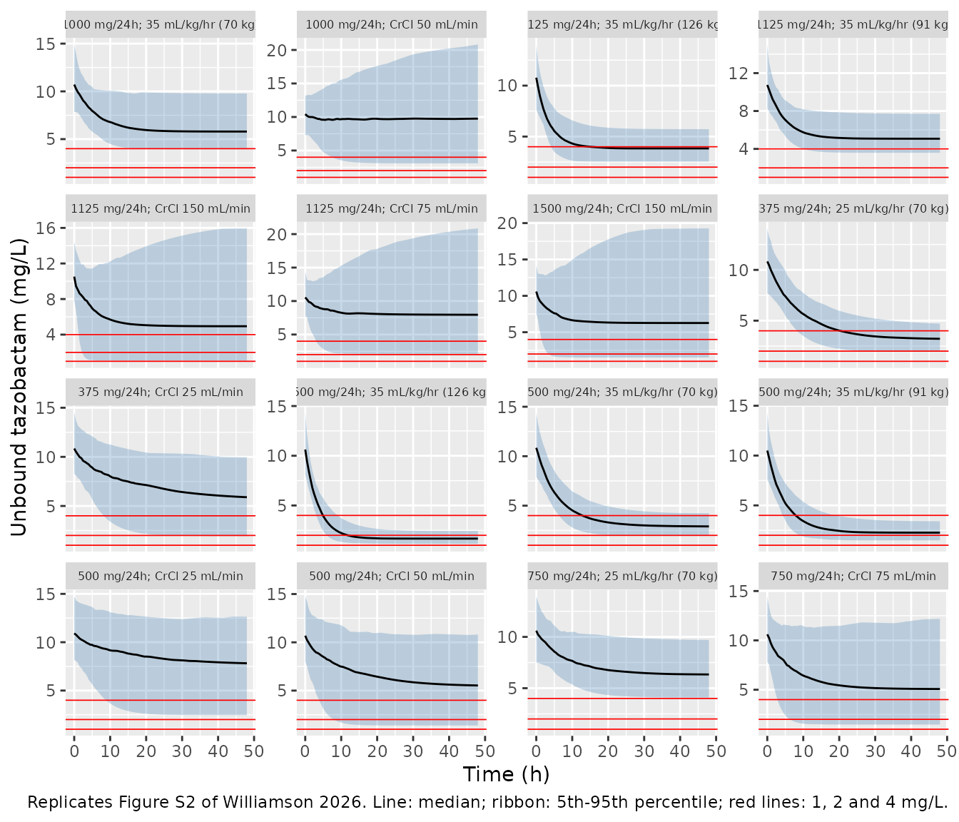
The medians at 48 h are compared with values read off the twelve Figure S2 panels (approximate to about 0.3 mg/L).
fig_s2 <- tibble::tribble(
  ~type,     ~stratum,                ~pub_median_48h,
  "High CI", "CrCl 50 mL/min",          10.5,
  "High CI", "35 mL/kg/hr (70 kg)",      5.3,
  "High CI", "CrCl 75 mL/min",           9.0,
  "Low CI",  "CrCl 150 mL/min",          4.8,
  "High CI", "CrCl 150 mL/min",          6.5,
  "Low CI",  "CrCl 25 mL/min",           6.5,
  "Low CI",  "25 mL/kg/hr (70 kg)",      2.8,
  "High CI", "CrCl 25 mL/min",           8.0,
  "Low CI",  "CrCl 50 mL/min",           5.3,
  "Low CI",  "35 mL/kg/hr (70 kg)",      2.8,
  "Low CI",  "CrCl 75 mL/min",           5.8,
  "High CI", "25 mL/kg/hr (70 kg)",      6.0
)

s2 <- sim |>
  dplyr::filter(time == 48) |>
  dplyr::group_by(type, stratum, dose) |>
  dplyr::summarise(sim_median_48h = median(Cu), .groups = "drop") |>
  dplyr::inner_join(fig_s2, by = c("type", "stratum")) |>
  dplyr::mutate(pct_diff = 100 * (sim_median_48h - pub_median_48h) / pub_median_48h)
stopifnot(nrow(s2) == nrow(fig_s2))

knitr::kable(
  s2 |>
    dplyr::rename("Regimen" = type, "Renal state" = stratum,
                  "Dose (mg/day)" = dose,
                  "Simulated median Cu at 48 h (mg/L)" = sim_median_48h,
                  "Figure S2 median (mg/L)" = pub_median_48h,
                  "% difference" = pct_diff),
  digits = 1,
  caption = "Median unbound concentration at 48 h, simulated vs. Figure S2."
)| Regimen | Renal state | Dose (mg/day) | Simulated median Cu at 48 h (mg/L) | Figure S2 median (mg/L) | % difference |
|---|---|---|---|---|---|
| High CI | 25 mL/kg/hr (70 kg) | 750 | 6.3 | 6.0 | 5.6 |
| High CI | 35 mL/kg/hr (70 kg) | 1000 | 5.8 | 5.3 | 9.3 |
| High CI | CrCl 150 mL/min | 1500 | 6.3 | 6.5 | -3.6 |
| High CI | CrCl 25 mL/min | 500 | 7.8 | 8.0 | -2.2 |
| High CI | CrCl 50 mL/min | 1000 | 9.8 | 10.5 | -7.1 |
| High CI | CrCl 75 mL/min | 1125 | 8.0 | 9.0 | -11.6 |
| Low CI | 25 mL/kg/hr (70 kg) | 375 | 3.2 | 2.8 | 14.9 |
| Low CI | 35 mL/kg/hr (70 kg) | 500 | 2.9 | 2.8 | 3.8 |
| Low CI | CrCl 150 mL/min | 1125 | 4.9 | 4.8 | 3.0 |
| Low CI | CrCl 25 mL/min | 375 | 5.9 | 6.5 | -9.4 |
| Low CI | CrCl 50 mL/min | 500 | 5.5 | 5.3 | 4.4 |
| Low CI | CrCl 75 mL/min | 750 | 5.1 | 5.8 | -12.5 |
Replicate Figures 3 and 4: target attainment
Target attainment is the fraction of subjects whose unbound concentration stays above the threshold at every time point from 24 to 48 h.
pta <- sim |>
  dplyr::filter(time >= 24) |>
  dplyr::group_by(k, panel, stratum, type, id) |>
  dplyr::summarise(cmin = min(Cu), .groups = "drop") |>
  dplyr::group_by(k, panel, stratum, type) |>
  dplyr::summarise(`1` = 100 * mean(cmin > 1), `2` = 100 * mean(cmin > 2),
                   `4` = 100 * mean(cmin > 4), .groups = "drop") |>
  tidyr::pivot_longer(c(`1`, `2`, `4`), names_to = "threshold",
                      values_to = "sim_pta")

pta |>
  dplyr::mutate(stratum = factor(stratum, levels = renal$stratum),
                threshold = paste0("100% fT > ", threshold, " mg/L")) |>
  ggplot(aes(stratum, sim_pta, colour = type, group = type)) +
  geom_line() +
  geom_point() +
  geom_hline(yintercept = 90, linetype = "dashed") +
  facet_grid(panel ~ threshold, scales = "free_x") +
  scale_y_continuous(limits = c(0, 100)) +
  labs(x = NULL, y = "Probability of target attainment (%)", colour = "Regimen",
       caption = "Replicates Figures 3 (non-CRRT) and 4 (CRRT) of Williamson 2026.") +
  theme(axis.text.x = element_text(angle = 35, hjust = 1, size = 7))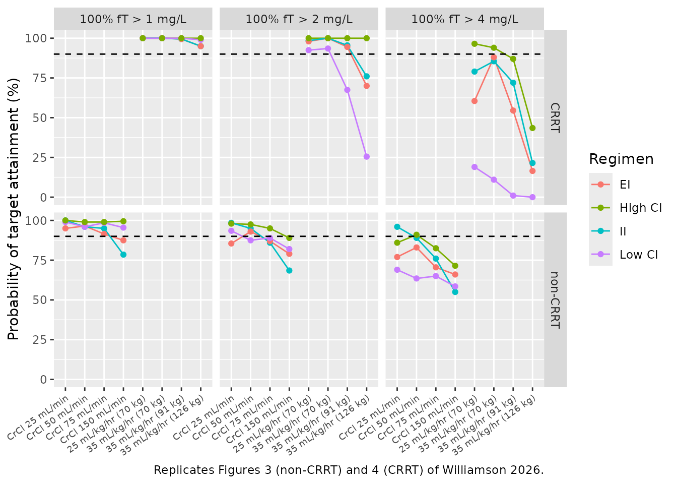
Comparison against the published percentages
Figures 3 and 4 have no numeric table behind them; the published values below are read off the plots (about +/- 3 percentage points), except the 88% that the Results text states for low-dose CI at CrCL 150 mL/min and 2 mg/L.
strata_order <- renal$stratum
published <- tibble::tribble(
  ~type,     ~threshold, ~v1, ~v2, ~v3, ~v4, ~v5, ~v6, ~v7, ~v8,
  "High CI", "1",        100, 100,  99,  98, 100, 100, 100, 100,
  "Low CI",  "1",         99,  99,  99,  99, 100,  99,  97,  84,
  "EI",      "1",         99,  99,  99,  99, 100, 100, 100,  99,
  "II",      "1",        100, 100,  99,  96, 100, 100, 100,  99,
  "High CI", "2",         99,  99,  98,  93, 100, 100, 100,  99,
  "Low CI",  "2",         97,  93,  94,  88,  94,  90,  83,  63,
  "EI",      "2",         99,  99,  98,  96,  99,  99,  99,  92,
  "II",      "2",         99,  99,  98,  92,  99,  99,  99,  93,
  "High CI", "4",         90,  93,  87,  76,  92,  89,  73,  16,
  "Low CI",  "4",         84,  70,  74,  60,   9,   4,   0,   0,
  "EI",      "4",         96,  97,  92,  83,  92,  97,  86,  59,
  "II",      "4",         99,  98,  95,  82,  95,  95,  92,  69
) |>
  tidyr::pivot_longer(v1:v8, names_to = "pos", values_to = "pub_pta") |>
  dplyr::mutate(stratum = strata_order[as.integer(sub("v", "", pos))]) |>
  dplyr::select(-pos)

cmp <- pta |>
  dplyr::inner_join(published, by = c("type", "stratum", "threshold")) |>
  dplyr::mutate(diff = sim_pta - pub_pta,
                stratum = factor(stratum, levels = strata_order)) |>
  dplyr::arrange(threshold, panel, type, stratum)
stopifnot(nrow(cmp) == 96L)

knitr::kable(
  cmp |>
    dplyr::filter(threshold == "4") |>
    dplyr::select(type, stratum, sim_pta, pub_pta, diff) |>
    dplyr::rename("Regimen" = type, "Renal state" = stratum,
                  "Simulated PTA (%)" = sim_pta,
                  "Figures 3/4 PTA (%)" = pub_pta, "Diff (pp)" = diff),
  digits = 1,
  caption = "Target attainment at the 4 mg/L threshold, simulated vs. published."
)| Regimen | Renal state | Simulated PTA (%) | Figures 3/4 PTA (%) | Diff (pp) |
|---|---|---|---|---|
| EI | 25 mL/kg/hr (70 kg) | 60.5 | 92 | -31.5 |
| EI | 35 mL/kg/hr (70 kg) | 88.0 | 97 | -9.0 |
| EI | 35 mL/kg/hr (91 kg) | 54.5 | 86 | -31.5 |
| EI | 35 mL/kg/hr (126 kg) | 16.5 | 59 | -42.5 |
| High CI | 25 mL/kg/hr (70 kg) | 96.5 | 92 | 4.5 |
| High CI | 35 mL/kg/hr (70 kg) | 94.0 | 89 | 5.0 |
| High CI | 35 mL/kg/hr (91 kg) | 87.0 | 73 | 14.0 |
| High CI | 35 mL/kg/hr (126 kg) | 43.5 | 16 | 27.5 |
| II | 25 mL/kg/hr (70 kg) | 79.0 | 95 | -16.0 |
| II | 35 mL/kg/hr (70 kg) | 85.5 | 95 | -9.5 |
| II | 35 mL/kg/hr (91 kg) | 72.0 | 92 | -20.0 |
| II | 35 mL/kg/hr (126 kg) | 21.5 | 69 | -47.5 |
| Low CI | 25 mL/kg/hr (70 kg) | 19.0 | 9 | 10.0 |
| Low CI | 35 mL/kg/hr (70 kg) | 11.0 | 4 | 7.0 |
| Low CI | 35 mL/kg/hr (91 kg) | 1.0 | 0 | 1.0 |
| Low CI | 35 mL/kg/hr (126 kg) | 0.0 | 0 | 0.0 |
| EI | CrCl 25 mL/min | 77.0 | 96 | -19.0 |
| EI | CrCl 50 mL/min | 83.0 | 97 | -14.0 |
| EI | CrCl 75 mL/min | 70.5 | 92 | -21.5 |
| EI | CrCl 150 mL/min | 66.0 | 83 | -17.0 |
| High CI | CrCl 25 mL/min | 86.0 | 90 | -4.0 |
| High CI | CrCl 50 mL/min | 91.0 | 93 | -2.0 |
| High CI | CrCl 75 mL/min | 82.5 | 87 | -4.5 |
| High CI | CrCl 150 mL/min | 71.5 | 76 | -4.5 |
| II | CrCl 25 mL/min | 96.0 | 99 | -3.0 |
| II | CrCl 50 mL/min | 89.0 | 98 | -9.0 |
| II | CrCl 75 mL/min | 76.0 | 95 | -19.0 |
| II | CrCl 150 mL/min | 55.0 | 82 | -27.0 |
| Low CI | CrCl 25 mL/min | 69.0 | 84 | -15.0 |
| Low CI | CrCl 50 mL/min | 63.5 | 70 | -6.5 |
| Low CI | CrCl 75 mL/min | 65.0 | 74 | -9.0 |
| Low CI | CrCl 150 mL/min | 58.5 | 60 | -1.5 |
cmp |>
  dplyr::group_by(Regimen = ifelse(grepl("CI", type), "Continuous infusion",
                                   "Intermittent / extended"),
                  Threshold = paste(threshold, "mg/L")) |>
  dplyr::summarise(`Median diff (pp)` = median(diff),
                   `Median abs diff (pp)` = median(abs(diff)),
                   .groups = "drop") |>
knitr::kable(digits = 1, caption = "Summary of simulated minus published PTA.")| Regimen | Threshold | Median diff (pp) | Median abs diff (pp) |
|---|---|---|---|
| Continuous infusion | 1 mg/L | 0.0 | 0.2 |
| Continuous infusion | 2 mg/L | -2.2 | 3.2 |
| Continuous infusion | 4 mg/L | -0.8 | 4.8 |
| Intermittent / extended | 1 mg/L | -3.2 | 3.2 |
| Intermittent / extended | 2 mg/L | -5.2 | 5.2 |
| Intermittent / extended | 4 mg/L | -19.0 | 19.0 |
cmp_ci <- cmp |> dplyr::filter(grepl("CI", type))
pta4 <- cmp |> dplyr::filter(threshold == "4")
hi_lo <- pta4 |>
  dplyr::filter(grepl("CI", type)) |>
  dplyr::select(stratum, type, sim_pta) |>
  tidyr::pivot_wider(names_from = type, values_from = sim_pta)

stopifnot(
  # The continuous-infusion arms depend only on clearance, and they reproduce:
  # 200 subjects per arm gives a Monte Carlo SE of up to ~3.5 pp, plus ~3 pp of
  # digitisation, so assert on the centre and a robust envelope.
  median(abs(cmp_ci$diff)) < 6,
  quantile(abs(cmp_ci$diff), 0.75) < 12,
  # Results: "all regimens failed to achieve the target for patients with
  # CrCL = 150 mL/min" at 4 mg/L.
  all(pta4$sim_pta[pta4$stratum == "CrCl 150 mL/min"] < 90),
  # Results: "The low-dose CI regimens failed to achieve >=90% target
  # attainment across all renal dispositions at a threshold target of 4 mg/L".
  all(pta4$sim_pta[pta4$type == "Low CI"] < 90),
  # "the high-dose CI regimens generally performed better": in every stratum.
  all(hi_lo$`High CI` > hi_lo$`Low CI`),
  # Results: all CI regimens >= 90% at 1 mg/L off CRRT.
  all(cmp_ci$sim_pta[cmp_ci$threshold == "1" & cmp_ci$panel == "non-CRRT"] >= 90)
)
The continuous-infusion arms reproduce Figures 3 and 4 to within a few percentage points at the centre; the largest continuous-infusion difference is the high-dose arm on CRRT in heavier patients at 4 mg/L, which the paper shows lower than this simulation (Figure 4: 73% at 91 kg and 16% at 126 kg). The intermittent (II) and extended (EI) infusion arms do not: the paper reports these as markedly more successful than the model, as transcribed, can produce from the Table S2 regimens – most visibly at 4 mg/L on CRRT, where Figure 4 shows 59-69% attainment for 126 kg patients against roughly 15-25% here. Because the same parameters reproduce the continuous-infusion arms and the Figure S2 concentration medians, which pin down clearance and the unbound fraction, and because the initial Figure S2 peak pins the volume, the gap is in how the published intermittent-regimen simulations were set up rather than in the model parameters. See the Assumptions section.
Sensitivity: the alternative reading of the IIV percentages
Table 1 reports interindividual variability as “C.V. %”, which this
model converts with omega^2 = log(1 + CV^2). Read instead
as Monolix omega standard deviations (omega^2 = CV^2), the
renal-arm variance rises from 0.96 to 1.61; the other two barely change.
The continuous-infusion arms off CRRT, where the renal arm acts, move
away from the published values under that reading:
mod_sd <- mod |>
  rxode2::ini(etalvc ~ 0.190^2, etalcl_renal ~ 1.27^2, etalcl_crrt ~ 0.261^2)
#> ℹ parameter labels from comments will be replaced by 'label()'
#> ℹ change initial estimate of `etalvc` to `0.0361`
#> ℹ change initial estimate of `etalcl_renal` to `1.6129`
#> ℹ change initial estimate of `etalcl_crrt` to `0.068121`
ci_off <- regimens$k[regimens$is_ci & regimens$panel == "non-CRRT"]
sim_sd <- rxode2::rxSolve(mod_sd, events = events |> dplyr::filter(k %in% ci_off),
                          keep = "k") |>
  as.data.frame()
pta_sd <- sim_sd |>
  dplyr::filter(time >= 24) |>
  dplyr::group_by(k, id) |>
  dplyr::summarise(cmin = min(Cu), .groups = "drop") |>
  dplyr::group_by(k) |>
  dplyr::summarise(`1` = 100 * mean(cmin > 1), `2` = 100 * mean(cmin > 2),
                   `4` = 100 * mean(cmin > 4), .groups = "drop") |>
  tidyr::pivot_longer(-k, names_to = "threshold", values_to = "sim_pta_sd")

sens <- cmp |>
  dplyr::filter(k %in% ci_off) |>
  dplyr::inner_join(pta_sd, by = c("k", "threshold")) |>
  dplyr::summarise(
    `Median abs diff, log(1 + CV^2) (pp)` = median(abs(sim_pta - pub_pta)),
    `Median abs diff, CV^2 (pp)` = median(abs(sim_pta_sd - pub_pta))
  )
knitr::kable(sens, digits = 1,
caption = "Off-CRRT continuous-infusion arms, both IIV readings.")| Median abs diff, log(1 + CV^2) (pp) | Median abs diff, CV^2 (pp) |
|---|---|
| 3.2 | 7.5 |
PKNCA validation
The paper reports no non-compartmental parameters. PKNCA is used for
the strongest structural check the model admits: after a single 500 mg
IV bolus, AUC(0-inf) must equal Dose / CL and
the half-life ln(2) * Vc / CL for every simulated
subject.
n_nca <- 200L
nca_events <- tibble::tibble(
  id = seq_len(n_nca), CRCL = 120, RRT_CRRT_ACTIVE = 0,
  RRT_HEMODIAL_ACTIVE = 0, RRT_CRRT_EFFLUENT_FLOW = 0,
  treatment = "500 mg IV bolus, CrCL 120 mL/min"
) |>
  (\(covs) dplyr::bind_rows(
    covs |> dplyr::mutate(time = 0, amt = 500, evid = 1L, cmt = "central"),
    covs |> tidyr::crossing(time = c(seq(0, 8, by = 0.25), seq(8.5, 24, by = 0.5))) |>
      dplyr::mutate(amt = NA_real_, evid = 0L, cmt = "central")
  ))() |>
  dplyr::arrange(id, time, dplyr::desc(evid))

nca_sim <- rxode2::rxSolve(mod, events = nca_events, keep = "treatment",
                          rtol = 1e-10, atol = 1e-12) |>
  as.data.frame()

# Keep each profile down to 1e-6 of its own peak, so the log-linear half-life
# fit does not follow integrator noise for the fastest-clearing subjects.
sim_nca <- nca_sim |>
  dplyr::filter(!is.na(Cc)) |>
  dplyr::group_by(id) |>
  dplyr::filter(Cc >= 1e-6 * max(Cc)) |>
  dplyr::ungroup() |>
  dplyr::select(id, time, Cc, treatment)

conc_obj <- PKNCA::PKNCAconc(sim_nca, Cc ~ time | treatment + id)
dose_obj <- PKNCA::PKNCAdose(
  nca_events |> dplyr::filter(evid == 1) |> dplyr::select(id, time, amt, treatment),
  amt ~ time | treatment + id
)
intervals <- data.frame(start = 0, end = Inf, cmax = TRUE, tmax = TRUE,
                        aucinf.obs = TRUE, half.life = TRUE)
nca_res <- PKNCA::pk.nca(PKNCA::PKNCAdata(conc_obj, dose_obj, intervals = intervals))

ident <- as.data.frame(nca_res) |>
  dplyr::filter(PPTESTCD %in% c("aucinf.obs", "cmax", "half.life")) |>
  dplyr::select(id, PPTESTCD, PPORRES) |>
  tidyr::pivot_wider(names_from = PPTESTCD, values_from = PPORRES) |>
  dplyr::mutate(id = as.integer(as.character(id))) |>
  dplyr::inner_join(
    nca_sim |> dplyr::group_by(id) |>
      dplyr::summarise(cl = dplyr::first(cl), vc = dplyr::first(vc), .groups = "drop"),
    by = "id"
  ) |>
  dplyr::mutate(
    auc_pct_diff = 100 * (aucinf.obs - 500 / cl) / (500 / cl),
    cmax_pct_diff = 100 * (cmax - 500 / vc) / (500 / vc),
    thalf_pct_diff = 100 * (half.life - log(2) * vc / cl) / (log(2) * vc / cl)
  )
stopifnot(nrow(ident) == n_nca)

knitr::kable(
  tibble::tibble(
    Identity = c("AUC(0-inf) = Dose / CL", "Cmax = Dose / Vc",
                 "t-half = ln(2) * Vc / CL"),
    `Max abs % difference` = formatC(c(max(abs(ident$auc_pct_diff)),
                                       max(abs(ident$cmax_pct_diff)),
                                       max(abs(ident$thalf_pct_diff))),
                                     format = "e", digits = 1)
  ),
  caption = paste("Per-subject structural identities across", n_nca, "subjects.")
)| Identity | Max abs % difference |
|---|---|
| AUC(0-inf) = Dose / CL | 1.5e-08 |
| Cmax = Dose / Vc | 0.0e+00 |
| t-half = ln(2) * Vc / CL | 1.9e-08 |
knitr::kable(
  ident |>
    dplyr::summarise(dplyr::across(c(cmax, aucinf.obs, half.life),
                                   list(median = median, p05 = ~ quantile(.x, 0.05),
                                        p95 = ~ quantile(.x, 0.95)))) |>
    tidyr::pivot_longer(dplyr::everything(),
                        names_to = c("parameter", "stat"), names_sep = "_") |>
    tidyr::pivot_wider(names_from = stat, values_from = value) |>
    dplyr::mutate(parameter = dplyr::recode(
      parameter, cmax = "Cmax (mg/L)", aucinf.obs = "AUC0-inf (obs) (mg*h/L)",
      half.life = "t1/2 (h)")) |>
    dplyr::rename("NCA parameter" = parameter, "Median" = median,
                  "5th percentile" = p05, "95th percentile" = p95),
  digits = 2,
  caption = "Simulated total-tazobactam NCA after 500 mg IV at CrCL 120 mL/min."
)| NCA parameter | Median | 5th percentile | 95th percentile |
|---|---|---|---|
| Cmax (mg/L) | 15.16 | 11.48 | 19.80 |
| AUC0-inf (obs) (mg*h/L) | 88.05 | 21.11 | 255.16 |
| t1/2 (h) | 3.79 | 0.90 | 12.27 |
Assumptions and deviations
-
IIV conversion. Table 1 gives interindividual
variability as “C.V. %” with the footnote “reported as CV % based on the
standard deviation of the random effects”. Monolix reports omega as a
standard deviation, so the percentages could be omega x 100
(
omega^2 = CV^2) or a log-normal CV (omega^2 = log(1 + CV^2)). The two readings differ materially only for the renal arm (127%: variance 1.61 vs 0.96). This model useslog(1 + CV^2), the convention of the companion piperacillin model from the same authors and cohort, and the reading under which the continuous-infusion target attainment sits closer to Figure 3 (sensitivity table above). -
Residual error is Monolix “combined1” (SD = a + b *
prediction), per Table S1’s “y2 comb1” for tazobactam, encoded with
combined1(). -
Unbound fraction. The model was fitted to total
tazobactam. The 70% unbound fraction is a literature value (Zosyn label,
reference 12) that the authors applied only in the simulations; it is
carried as the fixed parameter
fuand the outputCu, which are not part of the fitted model. - The intermittent and extended infusion arms do not reproduce Figures 3 and 4. Simulated attainment for II and EI regimens is lower than published, by up to about 45 percentage points (CRRT, 126 kg, 4 mg/L). The continuous infusion arms and the Figure S2 medians, which use the same clearance and unbound fraction, do reproduce, so no parameter in the model can close the gap without breaking those. The paper does not describe the timing of the maintenance doses relative to the loading dose, the infusion duration of the loading dose, or the time grid on which 100% fT > threshold was evaluated; none of the plausible choices tried (first maintenance dose at time zero or one interval after the loading dose) changes attainment at 24-48 h by more than a few percentage points. The model is used as published, without adjustment.
- Dosing design choices. The 500 mg loading dose is given as an IV bolus at time zero (the initial Figure S2 peak of about 10 mg/L unbound, i.e. 0.7 x 500 / 32.8, is consistent with a bolus). Continuous infusions start at time zero; intermittent and extended maintenance doses start one dosing interval after the loading dose.
-
Effluent flow units. The prose after Equation 6
gives FLOW “in mL/h”, normalised by 2 L/h. The canonical
RRT_CRRT_EFFLUENT_FLOWcolumn is in mL/h andmodel()divides by 2000. Weight-normalised prescriptions must be multiplied by body weight first; the Methods’ “25 and 35 L/kg/h” is a typo for mL/kg/h (the Results and Table S2 use mL/kg/hr). - Intra-hemodialysis clearance is fixed, not estimated (5.68 L/h from reference 22), because only one patient received intermittent hemodialysis and sampling did not align with dialysis sessions. No simulated regimen activates it.
- The Equation 5 gate switches off the non-renal arm too. On CRRT or hemodialysis, total clearance is the CRRT or hemodialysis arm alone, as the Results state (“equal to CRRT or HD CL when on renal replacement”).
- Cockcroft-Gault CrCL on renal replacement. The value is inert under the gate; this vignette supplies a non-zero placeholder (15 mL/min) so that a broken gate would fail an assertion.
- The Discussion’s 4.38 L/h for “total TAZ clearance in our cohort for the average CrCL” is not reproduced from the Table 1 values at the reported mean CrCL of 78 mL/min (4.9 x 78 / 120 + 0.91 = 4.10 L/h); it may be a mean of individual estimates. It is not used by the model.
- Cohort size. The paper simulated 1,000 patients per regimen and sampled parameter uncertainty from the full covariance matrix; this vignette uses 200 per arm (the library cap) and the point estimates only.
- Below-quantitation samples. Four of 162 observations were below the 0.5 mg/L LLOQ and were interval-censored in Monolix; censoring affects estimation only.