Posaconazole (Dvorackova 2023)
Source:vignettes/articles/Dvorackova_2023_posaconazole.Rmd
Dvorackova_2023_posaconazole.RmdModel and source
- Citation: Dvorackova E, Sima M, Zajacova A, Vyskocilova K, Kotowski T, Dunovska K, Klapkova E, Havlin J, Lischke R, Slanar O. Dosing Optimization of Posaconazole in Lung-Transplant Recipients Based on Population Pharmacokinetic Model. Antibiotics (Basel). 2023;12(9):1399. doi:10.3390/antibiotics12091399.
- Description: Population PK model for oral posaconazole tablets in adult lung-transplant recipients (Dvorackova 2023). One-compartment disposition with first-order absorption and first-order elimination, parameterised on the apparent (oral) scale as CL/F and Vd/F because bioavailability was not identifiable from the oral-only therapeutic-drug-monitoring data. The absorption rate constant Ka was fixed to 0.8 1/h (back-calculated from the tmax and half-life reported in the posaconazole SmPC) because all concentrations were sampled in the elimination phase; inter-individual variability on Ka was nevertheless estimated and is very large, reflecting that absorption is essentially unidentifiable from these data. Age is the only covariate retained in the final model, entering log-linearly (exponentially) on apparent clearance so that CL/F declines by about 0.9 percent per year of age. Residual variability is proportional. The model was used for Monte Carlo dose optimisation against the EUCAST trough targets of 0.7 mg/L for prophylaxis and 1.25 mg/L for therapy.
- Article: https://doi.org/10.3390/antibiotics12091399
Dvorackova and colleagues developed the first population pharmacokinetic model of posaconazole tablets in lung-transplant recipients, and used it to propose an age-banded dosing regimen replacing the approved uniform 300 mg once-daily dose. A one-compartment model with first-order absorption and first-order elimination described the data. Because posaconazole was given only orally, bioavailability was not identifiable and the disposition parameters are apparent values, CL/F and Vd/F.
Population
Thirty-two adult lung-transplant recipients (10 female, 22 male) treated at Motol University Hospital, Prague, between October 2020 and March 2023 contributed 80 serum posaconazole concentrations (1-12 per patient, mean 2.5, mode 2) collected as part of routine therapeutic drug monitoring. Median age was 56 years (IQR 48-61, range 22-71), median body weight 69 kg (IQR 60-83, range 38-100), and median CKD-EPI eGFR 0.98 mL/s/1.73 m2 (Dvorackova 2023 Table 1). Indications for transplantation were interstitial lung disease (13), idiopathic pulmonary fibrosis or other fibrotic change (7), COPD (7), cystic fibrosis (3), bronchial asthma (1), and chronic aspergillosis (1). All patients received maintenance immunosuppression (tacrolimus in 31, cyclosporin A in 1, plus prednisone in all and mycophenolate mofetil in 31), and 29 of 32 took a gastric-pH-raising drug.
Posaconazole was started at 300 mg once daily in every patient and subsequently adjusted by therapeutic drug monitoring over a range of 100-400 mg once daily. All samples were drawn in the elimination phase, from treatment day 4 onward (Dvorackova 2023 Section 4.2) – a fact that drives several of the model’s distinguishing features, discussed below.
The same information is available programmatically via the model’s
population metadata
(readModelDb("Dvorackova_2023_posaconazole")()$population).
pop <- readModelDb("Dvorackova_2023_posaconazole")()$population
str(pop[c("species", "n_subjects", "age_range", "weight_range", "dose_range")])
#> List of 5
#>  $ species     : chr "human"
#>  $ n_subjects  : int 32
#>  $ age_range   : chr "22-71 years (median 56, IQR 48-61; Dvorackova 2023 Table 1)"
#>  $ weight_range: chr "38-100 kg (median 69, IQR 60-83; Dvorackova 2023 Table 1)"
#>  $ dose_range  : chr "100-400 mg once daily oral posaconazole tablets; all patients started at 300 mg once daily and were subsequentl"| __truncated__
Source trace
The per-parameter origin is recorded as an in-file comment next to
each ini() entry in
inst/modeldb/specificDrugs/Dvorackova_2023_posaconazole.R.
The table below collects them in one place for review.
| Equation / parameter | Value | Source location |
|---|---|---|
lka (Ka, fixed) |
0.8 1/h | Table 2, Ka_pop, R.S.E. NA. Fixed, not estimated:
Section 4.4 step 1 states Ka was “fixed to a value of 0.8 h-1, which was
calculated from t1/2 and time to reach maximum plasma concentration
(tmax) values reported in SmPC” |
lvc (Vd/F) |
386.35 L | Table 2, Vd/F_pop, R.S.E. 48.1% |
lcl (CL/F at AGE = 0) |
8.8 L/h | Table 2, CL/F_pop, R.S.E. 32.0% |
e_age_cl |
-0.009 1/year | Table 2, beta_CL/F_age, R.S.E. 63.0% |
etalka |
var = 3.43^2 | Table 2, omega_Ka = 3.43 (SD of the log-scale random
effect), R.S.E. 27.5% |
etalvc |
var = 0.45^2 | Table 2, omega_Vd/F = 0.45, R.S.E. 47.7% |
etalcl |
var = 0.36^2 | Table 2, omega_CL/F = 0.36, R.S.E. 20.3% |
propSd |
0.29 | Table 2, “Error model parameters – Proportional”, R.S.E. 11.3% |
| One-compartment structure, linear absorption + elimination | n/a | Section 2.2 (structural model selection) and Section 4.4 step 1 |
log(Ka) = log(Ka_pop) + eta_Ka |
n/a | Section 2.2, first displayed equation |
log(Vd/F) = log(Vd/F_pop) + eta_Vd/F |
n/a | Section 2.2, second displayed equation |
log(CL/F) = log(CL/F_pop) + beta_CL/F_age * age + eta_CL/F |
n/a | Section 2.2, third displayed equation |
| Apparent (oral) parameterisation, no separate F term | n/a | Section 4.4 step 1: “the model estimates are the values of the apparent volume of distribution (Vd/F) and apparent clearance (CL/F), where F represents oral bioavailability” |
| Proportional residual error | n/a | Section 2.2 (selected over additive and combined) |
| Age is the only retained covariate | n/a | Table 3 (age on CL/F, p = 0.012; all other tested covariate-parameter pairs p > 0.05) |
| PK/PD targets 0.7 / 1.25 mg/L; AUC24 >= 25 mg*h/L | n/a | Section 4.5 and Section 2.3 |
| Published Monte Carlo AUC and PTA values used below | n/a | Section 2.3 |
The age-on-clearance covariate form
The paper describes the age effect two different ways, and they are not equivalent:
- The printed final-model equation (Section 2.2) is
log(CL/F) = log(CL/F_pop) + beta_CL/F_age * age + eta_CL/F, i.e. an exponential (log-linear) effect of uncentered age:CL/F = 8.8 * exp(-0.009 * AGE). - The abstract, Section 2.2 prose, and the Table 2 row label describe it additively: “CL/F of 8.8 L/h decreases by 0.009 L/h with each year of the patient’s age”, with Table 2 giving units of “L/h per year”.
The model file implements the printed equation, following the standing convention that a displayed equation supersedes prose. That choice is not merely conventional here – it is independently confirmed by the paper’s own Monte Carlo results.
# Dvorackova 2023 Section 2.3 reports median steady-state AUC24 at the proposed
# age-banded regimen. At steady state AUC_tau = dose / (CL/F), so each reported
# median implies a median CL/F for that subgroup.
implied <- tibble::tribble(
  ~subgroup,             ~dose_mg, ~auc_median,
  "Prophylaxis, <= 60 y",     300,          51,
  "Prophylaxis, > 60 y",      200,          40,
  "Therapy, <= 60 y",         400,          68,
  "Therapy, > 60 y",          300,          60
) |>
  mutate(
    implied_cl = dose_mg / auc_median,
    # Invert each candidate covariate form for the age that would produce it.
    age_if_exponential = -log(implied_cl / 8.8) / 0.009,
    age_if_additive    = (8.8 - implied_cl) / 0.009
  )

implied |>
  mutate(across(c(implied_cl, age_if_exponential, age_if_additive), \(x) round(x, 1))) |>
  dplyr::rename(
    "Subgroup"                = subgroup,
    "Dose (mg)"               = dose_mg,
    "Published median AUC24 (mg*h/L)" = auc_median,
    "Implied CL/F (L/h)"      = implied_cl,
    "Age if exponential (y)"  = age_if_exponential,
    "Age if additive (y)"     = age_if_additive
  ) |>
  knitr::kable(
    caption = paste(
      "Back-solving the two candidate covariate forms against the paper's own",
      "simulated AUC values. The exponential form implies plausible subgroup",
      "median ages; the additive form implies impossible ones."
    )
)| Subgroup | Dose (mg) | Published median AUC24 (mg*h/L) | Implied CL/F (L/h) | Age if exponential (y) | Age if additive (y) |
|---|---|---|---|---|---|
| Prophylaxis, <= 60 y | 300 | 51 | 5.9 | 44.8 | 324.2 |
| Prophylaxis, > 60 y | 200 | 40 | 5.0 | 62.8 | 422.2 |
| Therapy, <= 60 y | 400 | 68 | 5.9 | 44.8 | 324.2 |
| Therapy, > 60 y | 300 | 60 | 5.0 | 62.8 | 422.2 |
The exponential form implies subgroup median ages of roughly 45 and 63 years – entirely plausible for a cohort with overall median age 56 (IQR 48-61) split at 60 years, and internally consistent (the two prophylaxis/therapy pairs that share an age band back-solve to the same clearance, 300/51 = 400/68 = 5.88 and 200/40 = 300/60 = 5.00 L/h). The additive form implies median ages in the hundreds of years. Moreover, across the entire observed 22-71 year age range the additive form would move CL/F by only about 5% (8.60 to 8.16 L/h), far too little to motivate the paper’s 200/300/400 mg age-banded dosing proposal, whereas the exponential form moves it by about 36% (7.22 to 4.64 L/h).
Note the consequence for lcl: because age enters
uncentered, 8.8 L/h is the mathematical intercept at
AGE = 0, not a clearance attained by any subject. At the
cohort median age of 56 years the typical CL/F is
8.8 * exp(-0.009 * 56) = 5.32 L/h.
Virtual cohort
Individual patient data are not published, so the virtual cohort reconstructs the age distribution from the five order statistics reported in Dvorackova 2023 Table 1 (min 22, Q1 48, median 56, Q3 61, max 71) using a piecewise-linear quantile function. Age is the only covariate in the model, so no other covariate distribution is needed.
Three arms of 200 subjects each are simulated. All three share the
same age draw so that the regimen comparisons are paired and
free of age-sampling noise; IDs are offset so they remain disjoint
subjects for rxSolve.
set.seed(20230901)

n_per_arm <- 200L
tau       <- 24    # dosing interval (h)
n_days    <- 60L   # days of once-daily dosing before the evaluation interval
t_last    <- (n_days - 1L) * tau        # time of the final dose
t_end     <- t_last + tau               # end of the evaluation interval

# Piecewise-linear quantile function through the Table 1 order statistics.
age_quantile <- function(p) {
  stats::approx(
    x    = c(0, 0.25, 0.50, 0.75, 1),
    y    = c(22,  48,   56,   61, 71),
    xout = p
  )$y
}

ages <- age_quantile(stats::runif(n_per_arm))

# Verify the reconstruction reproduces the published summary statistics.
tibble::tibble(
  Statistic = c("Minimum", "Q1", "Median", "Q3", "Maximum"),
  Published = c(22, 48, 56, 61, 71),
  Simulated = round(as.numeric(stats::quantile(ages, c(0, 0.25, 0.5, 0.75, 1))), 1)
) |>
knitr::kable(caption = "Virtual-cohort age distribution vs Dvorackova 2023 Table 1.")| Statistic | Published | Simulated |
|---|---|---|
| Minimum | 22 | 22.1 |
| Q1 | 48 | 47.7 |
| Median | 56 | 55.6 |
| Q3 | 61 | 60.7 |
| Maximum | 71 | 70.9 |
# Observation grid: a coarse grid over the accumulation phase for the profile
# figure, then a fine grid over the final dosing interval for NCA.
obs_times <- sort(unique(c(
  seq(0, 504, by = 6),
  seq(528, t_last, by = tau),
  seq(t_last, t_end, by = 0.5)
)))

make_arm <- function(regimen, dose_fun, id_offset) {
  subj <- tibble::tibble(
    id       = id_offset + seq_len(n_per_arm),
    AGE      = ages,
    regimen  = regimen,
    age_band = ifelse(ages <= 60, "age <= 60 y", "age > 60 y")
  ) |>
    mutate(dose_mg = dose_fun(AGE))

  doses <- subj |>
    tidyr::crossing(time = seq(0, t_last, by = tau)) |>
    mutate(amt = dose_mg, evid = 1L, cmt = "depot")

  obs <- subj |>
    tidyr::crossing(time = obs_times) |>
    mutate(amt = NA_real_, evid = 0L, cmt = "central")

  bind_rows(doses, obs) |>
    arrange(id, time, desc(evid))
}

events <- bind_rows(
  make_arm("Proposed, prophylaxis",
           \(age) ifelse(age <= 60, 300, 200), id_offset =   0L),
  make_arm("Proposed, therapy",
           \(age) ifelse(age <= 60, 400, 300), id_offset = 200L),
  make_arm("Approved uniform 300 mg",
           \(age) rep(300, length(age)),       id_offset = 400L)
)

# Disjoint-ID guard: duplicate IDs across arms would be silently merged by
# rxSolve into a single subject receiving the summed dose. Assert that every id
# belongs to exactly one arm, and that the three arms partition the id space.
stopifnot(
  nrow(dplyr::distinct(events, id, regimen)) == 3L * n_per_arm,
  dplyr::n_distinct(events$id) == 3L * n_per_arm
)

events |>
  filter(evid == 1, time == 0) |>
  count(regimen, age_band, dose_mg) |>
  dplyr::rename("Regimen" = regimen, "Age band" = age_band,
                "Dose (mg once daily)" = dose_mg, "N subjects" = n) |>
knitr::kable(caption = "Virtual cohort: arms, age bands, and assigned doses.")| Regimen | Age band | Dose (mg once daily) | N subjects |
|---|---|---|---|
| Approved uniform 300 mg | age <= 60 y | 300 | 142 |
| Approved uniform 300 mg | age > 60 y | 300 | 58 |
| Proposed, prophylaxis | age <= 60 y | 300 | 142 |
| Proposed, prophylaxis | age > 60 y | 200 | 58 |
| Proposed, therapy | age <= 60 y | 400 | 142 |
| Proposed, therapy | age > 60 y | 300 | 58 |
Simulation
Because omega_Ka is very large (3.43 on the log scale),
the sampled absorption rate constants span many orders of magnitude. The
OMEGA matrix is therefore constructed and passed explicitly rather than
relying on whatever matrix a prior rxSolve call left
behind, and the returned subject count is asserted.
mod <- readModelDb("Dvorackova_2023_posaconazole")

# Explicit OMEGA (diagonal; the paper reports no eta correlations).
omega <- diag(c(etalka = 3.43^2, etalvc = 0.45^2, etalcl = 0.36^2))
dimnames(omega) <- list(c("etalka", "etalvc", "etalcl"),
                        c("etalka", "etalvc", "etalcl"))

sim <- rxode2::rxSolve(
  mod,
  events = events,
  omega  = omega,
  keep   = c("regimen", "age_band", "dose_mg", "AGE"),
  addDosing = FALSE
) |>
  as.data.frame()
#> ℹ parameter labels from comments will be replaced by 'label()'

# rxSolve has been observed to silently drop subjects; assert the count.
stopifnot(length(unique(sim$id)) == 3L * n_per_arm)
stopifnot(!anyNA(sim$Cc))

sim <- sim |>
  mutate(
    group = paste0(regimen, ", ", age_band),
    tad   = time - t_last          # time after the final dose
  )
Replicate published figures
Figure 4 – simulated concentration-time profiles at the proposed regimen
Dvorackova 2023 Figure 4 shows simulated posaconazole concentration versus time under the proposed age-banded regimen, with the median, percentile bands, and a horizontal line at the applicable PK/PD trough target.
targets <- tibble::tibble(
  regimen = c("Proposed, prophylaxis", "Proposed, therapy"),
  target  = c(0.7, 1.25)
)

sim |>
  filter(regimen != "Approved uniform 300 mg", time <= 504) |>
  group_by(regimen, age_band, time) |>
  summarise(
    Q05  = quantile(Cc, 0.050),
    Q275 = quantile(Cc, 0.275),
    Q50  = quantile(Cc, 0.500),
    Q725 = quantile(Cc, 0.725),
    Q95  = quantile(Cc, 0.950),
    .groups = "drop"
  ) |>
  ggplot(aes(time / 24)) +
  geom_ribbon(aes(ymin = Q05,  ymax = Q275), alpha = 0.20) +
  geom_ribbon(aes(ymin = Q275, ymax = Q50),  alpha = 0.35) +
  geom_ribbon(aes(ymin = Q50,  ymax = Q725), alpha = 0.35) +
  geom_ribbon(aes(ymin = Q725, ymax = Q95),  alpha = 0.20) +
  geom_line(aes(y = Q50), linewidth = 0.8) +
  geom_hline(data = targets, aes(yintercept = target),
             linetype = "dashed", colour = "firebrick") +
  facet_grid(regimen ~ age_band) +
  labs(
    x = "Time (days)", y = "Posaconazole serum concentration (mg/L)",
    title = "Figure 4 - proposed age-banded dosing regimen",
    caption = paste(
      "Replicates Figure 4 of Dvorackova 2023. Black line = median;",
      "bands = 5-27.5, 27.5-50, 50-72.5, 72.5-95th percentiles.",
      "Dashed line = PK/PD trough target (0.7 mg/L prophylaxis, 1.25 mg/L therapy)."
    )
  )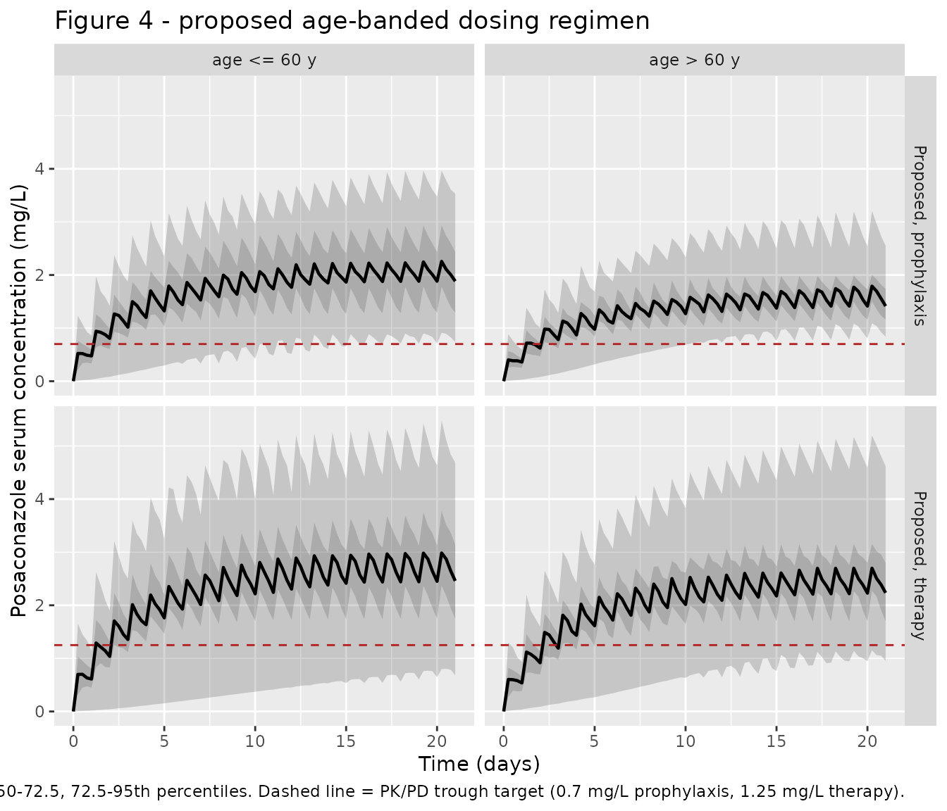
The profiles accumulate to steady state over roughly the first two weeks, and the median sits above the applicable target in all four panels – the qualitative result the paper’s Figure 4 reports.
PKNCA validation
Steady-state NCA is computed over the final dosing interval (AUC0-tau, Cmax, Tmax, and the end-of-interval trough at steady state).
The final dosing interval is rebased so that the last dose
sits at time 0 and the interval runs [0, tau]. This is not
cosmetic: PKNCA::pk.nca.interval() passes the concentration
times to each calculator relative to the interval start
(time - interval$start) but passes end as an
absolute value, so pk.calc.ctrough() –
which matches on time %in% end – can only resolve on an
interval that starts at 0. Verified against the installed PKNCA; on an
unrebased [t_last, t_end] interval every
ctrough comes back NA.
# Restrict to the final dosing interval and rebase it to [0, tau].
sim_nca <- sim |>
  filter(!is.na(Cc), time >= t_last, time <= t_end) |>
  mutate(time = time - t_last) |>
  select(id, time, Cc, group)

# The observation grid places a sample exactly at each interval boundary; assert
# it rather than patching a time-zero row in defensively, so a future change to
# the grid fails loudly instead of silently shifting the AUC baseline.
stopifnot(
  sum(sim_nca$time == 0)   == 3L * n_per_arm,
  sum(sim_nca$time == tau) == 3L * n_per_arm
)

conc_obj <- PKNCA::PKNCAconc(sim_nca, Cc ~ time | group + id,
                             concu = "mg/L", timeu = "h")

# One dose record per subject at the rebased time 0.
dose_df <- sim |>
  distinct(id, group, dose_mg) |>
  mutate(time = 0)

dose_obj <- PKNCA::PKNCAdose(dose_df, dose_mg ~ time | group + id, doseu = "mg")

intervals <- data.frame(
  start   = 0,
  end     = tau,
  cmax    = TRUE,
  tmax    = TRUE,
  auclast = TRUE,
  ctrough = TRUE   # PKNCA's "trough (end of interval) concentration"
)

nca_res <- PKNCA::pk.nca(PKNCA::PKNCAdata(conc_obj, dose_obj,
                                          intervals = intervals))

nca_long <- as.data.frame(nca_res)
Comparison against published simulated AUC
Dvorackova 2023 Section 2.3 reports the median (IQR) 24-hour AUC in each of the four proposed-regimen subgroups. Note that this is a simulation-versus-simulation comparison: the paper reports no NCA of observed concentrations, so the reference values are the summary statistics of the authors’ own Simulx Monte Carlo run.
published_auc <- tibble::tribble(
  ~group,                                    ~auclast,
  "Proposed, prophylaxis, age <= 60 y",            51,
  "Proposed, prophylaxis, age > 60 y",             40,
  "Proposed, therapy, age <= 60 y",                68,
  "Proposed, therapy, age > 60 y",                 60
)

sim_auc <- nca_long |>
  filter(PPTESTCD == "auclast", group %in% published_auc$group) |>
  select(group, PPTESTCD, PPORRES)

cmp <- nlmixr2lib::ncaComparisonTable(
  simulated     = sim_auc,
  reference     = published_auc,
  by            = "group",
  units         = c(auclast = "mg*h/L"),
  tolerance_pct = 20
)

knitr::kable(
  cmp,
  digits  = 1,
  caption = paste(
    "Steady-state AUC0-24: simulated median vs Dvorackova 2023 Section 2.3",
    "published median. * differs from reference by >20%."
  )
)| NCA parameter | group | Reference | Simulated | % diff |
|---|---|---|---|---|
| AUClast (mg*h/L) | Proposed, prophylaxis, age <= 60 y | 51 | 51.3 | +0.7% |
| AUClast (mg*h/L) | Proposed, prophylaxis, age > 60 y | 40 | 41.2 | +2.9% |
| AUClast (mg*h/L) | Proposed, therapy, age <= 60 y | 68 | 69.5 | +2.3% |
| AUClast (mg*h/L) | Proposed, therapy, age > 60 y | 60 | 60.6 | +1.0% |
attr(cmp, "footnote")
#> NULL
The published IQRs provide a second, distributional check.
nca_long |>
  filter(PPTESTCD == "auclast", group %in% published_auc$group) |>
  group_by(group) |>
  summarise(
    sim = sprintf("%.0f (%.0f-%.0f)",
                  median(PPORRES),
                  quantile(PPORRES, 0.25),
                  quantile(PPORRES, 0.75)),
    .groups = "drop"
  ) |>
  mutate(published = c("51 (39-66)", "40 (31-51)", "68 (52-89)", "60 (46-76)")) |>
  dplyr::rename(
    "Subgroup"                          = group,
    "Simulated AUC0-24, median (IQR)"   = sim,
    "Published AUC0-24, median (IQR)"   = published
  ) |>
  knitr::kable(
    caption = "Steady-state AUC0-24 (mg*h/L) distribution vs Dvorackova 2023 Section 2.3."
)| Subgroup | Simulated AUC0-24, median (IQR) | Published AUC0-24, median (IQR) |
|---|---|---|
| Proposed, prophylaxis, age <= 60 y | 51 (38-68) | 51 (39-66) |
| Proposed, prophylaxis, age > 60 y | 41 (33-49) | 40 (31-51) |
| Proposed, therapy, age <= 60 y | 70 (51-91) | 68 (52-89) |
| Proposed, therapy, age > 60 y | 61 (51-77) | 60 (46-76) |
Probability of target attainment
The paper’s central claim is that the proposed age-banded regimen
raises the probability of target attainment relative to the approved
uniform 300 mg dose. PTA is computed here from the steady-state trough
(ctau, the concentration at the end of the final dosing
interval) and from the steady-state AUC0-24.
ctau <- nca_long |>
  filter(PPTESTCD == "ctrough") |>
  select(id, group, ctau = PPORRES) |>
  mutate(id = as.integer(as.character(id)))

auc24 <- nca_long |>
  filter(PPTESTCD == "auclast") |>
  select(id, group, auc = PPORRES) |>
  mutate(id = as.integer(as.character(id)))

# ctau and auc are one row per subject; joining NCA output onto a per-subject
# table is the legitimate post-rxSolve join case.
pta_data <- ctau |>
  inner_join(auc24, by = c("id", "group")) |>
  inner_join(
    sim |> distinct(id, regimen, age_band, AGE),
    by = "id"
  )

pta <- function(data, indication) {
  thr <- if (indication == "prophylaxis") 0.7 else 1.25
  100 * mean(data$ctau > thr)
}

pta_table <- tibble::tribble(
  ~scenario,                                            ~published,
  "Proposed regimen, prophylaxis target (all ages)",           95,
  "Proposed regimen, therapy target (all ages)",               90,
  "Proposed regimen, therapy target, age > 60 y",              89,
  "Approved 300 mg uniform, prophylaxis target (all ages)",    96,
  "Approved 300 mg uniform, therapy target (all ages)",        81,
  "Approved 300 mg uniform, therapy target, age <= 60 y",      79
) |>
  mutate(
    simulated = c(
      pta(filter(pta_data, regimen == "Proposed, prophylaxis"), "prophylaxis"),
      pta(filter(pta_data, regimen == "Proposed, therapy"), "therapy"),
      pta(filter(pta_data, regimen == "Proposed, therapy",
                 age_band == "age > 60 y"), "therapy"),
      pta(filter(pta_data, regimen == "Approved uniform 300 mg"), "prophylaxis"),
      pta(filter(pta_data, regimen == "Approved uniform 300 mg"), "therapy"),
      pta(filter(pta_data, regimen == "Approved uniform 300 mg",
                 age_band == "age <= 60 y"), "therapy")
    ),
    difference = simulated - published
  )

pta_table |>
  mutate(across(c(simulated, difference), \(x) round(x, 0))) |>
  dplyr::rename(
    "Scenario"                = scenario,
    "Published PTA (%)"       = published,
    "Simulated PTA (%)"       = simulated,
    "Difference (pp)"         = difference
  ) |>
  knitr::kable(
    caption = paste(
      "Trough-based probability of target attainment vs Dvorackova 2023",
      "Section 2.3 (prophylaxis target Ctrough > 0.7 mg/L;",
      "therapy target Ctrough > 1.25 mg/L)."
    )
)| Scenario | Published PTA (%) | Simulated PTA (%) | Difference (pp) |
|---|---|---|---|
| Proposed regimen, prophylaxis target (all ages) | 95 | 98 | 4 |
| Proposed regimen, therapy target (all ages) | 90 | 92 | 2 |
| Proposed regimen, therapy target, age > 60 y | 89 | 93 | 4 |
| Approved 300 mg uniform, prophylaxis target (all ages) | 96 | 97 | 1 |
| Approved 300 mg uniform, therapy target (all ages) | 81 | 86 | 4 |
| Approved 300 mg uniform, therapy target, age <= 60 y | 79 | 82 | 3 |
The paper also evaluated the primary PK/PD index, AUC/MIC > 200 at the EUCAST Aspergillus breakpoint MIC of 0.125 mg/L, which corresponds to a 24-hour AUC of at least 25 mg*h/L.
tibble::tibble(
  Scenario = c("Proposed regimen, prophylaxis arm",
               "Proposed regimen, therapy arm",
               "Proposed regimen, both arms pooled"),
  Published = c(93, 98, 95),
  Simulated = round(c(
    100 * mean(filter(pta_data, regimen == "Proposed, prophylaxis")$auc >= 25),
    100 * mean(filter(pta_data, regimen == "Proposed, therapy")$auc >= 25),
    100 * mean(filter(pta_data, regimen != "Approved uniform 300 mg")$auc >= 25)
  ), 0)
) |>
  dplyr::rename(
    "Published PTA (%)" = Published,
    "Simulated PTA (%)" = Simulated
  ) |>
  knitr::kable(
    caption = paste(
      "AUC/MIC probability of target attainment (AUC0-24 >= 25 mg*h/L)",
      "vs Dvorackova 2023 Section 2.3."
    )
)| Scenario | Published PTA (%) | Simulated PTA (%) |
|---|---|---|
| Proposed regimen, prophylaxis arm | 93 | 94 |
| Proposed regimen, therapy arm | 98 | 98 |
| Proposed regimen, both arms pooled | 95 | 96 |
Observed trough concentrations at treatment initiation
Dvorackova 2023 Section 3 reports that the median (IQR) posaconazole serum level measured after treatment initiation, before any TDM-driven dose adjustment and therefore all at the starting dose of 300 mg once daily, was 1.61 (1.23-2.49) mg/L. This is the paper’s only summary of observed concentrations and provides an external check on the uniform-dose arm.
sim_trough <- pta_data |>
  filter(regimen == "Approved uniform 300 mg") |>
  summarise(
    q25 = quantile(ctau, 0.25),
    q50 = median(ctau),
    q75 = quantile(ctau, 0.75)
  )

tibble::tibble(
  Source = c("Observed (Dvorackova 2023 Section 3)", "Simulated (this vignette)"),
  `Trough at 300 mg once daily, median (IQR) mg/L` = c(
    "1.61 (1.23-2.49)",
    sprintf("%.2f (%.2f-%.2f)", sim_trough$q50, sim_trough$q25, sim_trough$q75)
  )
) |>
knitr::kable(caption = "Steady-state trough at the approved uniform dose.")| Source | Trough at 300 mg once daily, median (IQR) mg/L |
|---|---|
| Observed (Dvorackova 2023 Section 3) | 1.61 (1.23-2.49) |
| Simulated (this vignette) | 1.99 (1.50-2.77) |
Assumptions and deviations
-
Age-on-clearance covariate form. The paper states
the effect additively in prose (and in the Table 2 units column, “L/h
per year”) but writes it log-linearly in the displayed final-model
equation. The model file implements the displayed equation,
CL/F = 8.8 * exp(-0.009 * AGE). The Source trace section above shows the arithmetic confirming this against the paper’s own simulated AUC values; the additive reading is refuted by them. The Table 2 units label “L/h per year” is dimensionally inconsistent with the displayed equation, in whichbeta_CL/F_agehas units of 1/year. -
Uncentered age. Age enters uncentered, so
lcl = log(8.8)is the extrapolated intercept atAGE = 0, not a clearance any subject attains. Users should not extrapolate the model outside the observed 22-71 year range. - Age distribution. Individual ages are not published. The virtual cohort’s ages are drawn from a piecewise-linear quantile function through the five order statistics of Dvorackova 2023 Table 1; the reconstruction reproduces those five statistics (table in the Virtual cohort section). The paper’s own Monte Carlo instead resampled the 32 actual patients (500 replicates, 16,000 simulations), so the two age distributions are similar but not identical. Back-solving the published AUCs implies subgroup median ages of about 45 and 63 years, whereas the reconstruction gives about 51 and 65; this is the dominant source of the residual difference in the AUC comparison table and biases the simulated AUCs slightly upward in the younger band.
-
Very large IIV on Ka.
omega_Ka = 3.43is encoded faithfully rather than trimmed. All observed concentrations were drawn in the elimination phase from day 4 onward, so absorption is essentially unidentifiable from these data and the model reports that fact as an enormous random effect. Two practical consequences are visible in this vignette: roughly one subject in eight draws akabelow the elimination rate constant and is therefore in flip-flop kinetics, and a small minority draw akaso low that they have not reached steady state even after 60 days of once-daily dosing. Neither affects the structural steady-state relationshipAUC_tau = dose / (CL/F), which is independent ofka, but both widen the simulated trough distribution relative to what a better-identified absorption model would give. Anyone refitting this model to data that capture the absorption phase should expect to re-estimate bothlkaandetalka. -
Steady state. The paper does not state the
simulation horizon used for its Monte Carlo AUC and PTA values. This
vignette doses once daily for 60 days and evaluates the final dosing
interval; with a typical elimination half-life near 50 hours that is
comfortably at steady state for all but the extreme low-
katail described above. -
Ka fixed from the SmPC.
Ka = 0.8 1/hwas not estimated from the study data; the authors back-calculated it from the tmax and half-life in the posaconazole Summary of Product Characteristics (Section 4.4 step 1). It is encoded withfixed()to preserve that provenance. - Residual error in the simulation. The figures and NCA use the model’s structural predictions with between-subject variability but without residual error added, matching the paper’s Monte Carlo presentation of concentration profiles and derived exposure metrics.
-
Age band boundary. The paper describes its bands
variously as “under 60” / “up to 60” and “over 60”. This vignette uses
AGE <= 60andAGE > 60throughout. Because age is continuous in the model, the choice affects only which subjects fall in which reported subgroup, not any individual prediction. -
Covariates screened but not retained. Sex,
indication for transplantation, cystic fibrosis, calcineurin inhibitor,
mycophenolate mofetil, gastric-pH- raising drugs, height, body weight,
BMI, BSA, serum creatinine, eGFR, ALT, AST, and GGT were all tested and
none reached significance (Dvorackova 2023 Table 3). They are not
carried in
covariateDatabecause the model does not use them. - No erratum. No erratum, corrigendum, or author correction to doi:10.3390/antibiotics12091399 was located; the values above are from the original publication.
- Simulation-versus-simulation comparison. The paper publishes no NCA of observed concentrations, so the AUC and PTA reference values above are the authors’ own Monte Carlo summaries rather than independent observed data. The only observed-data anchor available is the median (IQR) trough at treatment initiation, compared in the last table.