Lopinavir in pregnancy (Fauchet 2015)
Source:vignettes/articles/Fauchet_2015_lopinavir.Rmd
Fauchet_2015_lopinavir.RmdModel and source
Fauchet et al. fit two parallel non-hierarchical popPK submodels for total and unbound lopinavir (LPV) in 208 HIV-infected women across the ANRS 135 PRIMEVA randomised trial and the Hospital Cochin therapeutic-drug-monitoring (TDM) cohort:
- an unbound submodel (Table 2) that ties total to unbound LPV via a linear human-serum-albumin (HSA / ALB) binding term plus a saturable single-site alpha-1 acid glycoprotein (AAG) binding term;
- a maternal-fetal-amniotic (MFLA) submodel (Table 4) that adds a placental-transfer effect compartment for cord-blood LPV and a downstream amniotic-fluid compartment, with a 39% multiplicative pregnancy effect on apparent maternal clearance.
Both submodels share a one-compartment first-order-absorption
disposition for maternal LPV. Per the standing extract-literature-model
policy of replicating the author’s structure, the two are packaged as
two separate model files (Fauchet_2015_lopinavir_unbound,
Fauchet_2015_lopinavir_placental) under one vignette.
- Citation: Fauchet F, Treluyer JM, Illamola SM, Pressiat C, Lui G, Valade E, Mandelbrot L, Lechedanec J, Delmas S, Blanche S, Warszawski J, Urien S, Tubiana R, Hirt D, for the ANRS 135 PRIMEVA Study Group. Population approach to analyze the pharmacokinetics of free and total lopinavir in HIV-infected pregnant women and consequences for dose adjustment. Antimicrob Agents Chemother. 2015;59(9):5727-5735.
- Article: https://doi.org/10.1128/AAC.00863-15
Population
The pooled cohort included 103 women from the ANRS 135 PRIMEVA randomised trial (69 LPV/r monotherapy at 400/100 mg BID and 34 LPV/r + zidovudine/lamivudine triple therapy at 400/100 + 300/150 mg BID) and 105 women from the Hospital Cochin (Paris) TDM service (81 pregnant, 24 nonpregnant). Median (range) body weight was 76 kg (45-122), median age was 31.2 years (18.3-44.3), and median sampled gestational age was 33 weeks (9-41). All TDM women received the standard 400/100 mg BID regimen in combination with zidovudine/lamivudine. The unbound submodel was fit against 400 maternal LPV concentrations, 79 of which had a paired unbound-LPV ultrafiltrate measurement; the MFLA submodel was fit against the same 400 maternal samples plus 79 cord-blood samples and 48 amniotic-fluid samples. Demographics from Table 1 of the source paper.
The same information is available programmatically via
readModelDb("Fauchet_2015_lopinavir_unbound")$population
and
readModelDb("Fauchet_2015_lopinavir_placental")$population.
Source trace
Per-parameter origins are recorded as in-file comments in the two model files; the tables below collect them for review.
Unbound submodel (Table 2). All values from Fauchet 2015 Table 2 (‘Population pharmacokinetic parameters of lopinavir from the unbound fraction model’). Sigmas are reported as proportional residual-error fractions and omega as the square root of between-subject variance.
| Parameter | Value | Source location |
|---|---|---|
lka (log Ka, 1/h) |
log(0.408) | Table 2 row Ka |
lcl (log apparent unbound CL/F, L/h) |
log(316) | Table 2 row CL |
lvc (log apparent unbound V/F, L) |
log(2220) | Table 2 row V |
lkhsa (log K_HSA, L/umol; linear HSA term) |
log(0.036) | Table 2 row K_HSA |
lkaag (log K_AAG, umol/L; saturable AAG
dissociation) |
log(0.159) | Table 2 row N_AAG K_AAG |
naag (LPV binding sites on AAG, fixed) |
1 | Table 2 footnote c; Results paragraph ‘The N_AAG value was fixed to 1 in the final model’ |
etalcl variance |
0.228^2 = 0.052 | Table 2 row omega_Cl (SD form) |
propSd (total LPV) |
0.450 | Table 2 row sigma_total |
propSd_Cunbound |
0.282 | Table 2 row sigma_unbound |
| Linear HSA + saturable AAG binding equation | n/a | Appendix equation 2 |
MFLA submodel (Table 4). Ka was fixed because the data did not support estimation; Fauchet 2015 used the value reported in Bouillon-Pichault et al. 2011 (reference 37 in the source paper).
| Parameter | Value | Source location |
|---|---|---|
lka (log Ka, 1/h, fixed) |
log(0.255) | Table 4 row Ka, footnote c; Results ‘MFLA model’ paragraph |
lcl (log nonpregnant apparent maternal CL/F, L/h) |
log(4.12) | Table 4 row CL |
lvc (log apparent maternal V/F, L) |
log(43.1) | Table 4 row V |
lk1f (log maternal-to-fetal rate, 1/h) |
log(0.035) | Table 4 row K_1F |
lkfla (log fetal-to-amniotic rate, 1/h) |
log(0.289) | Table 4 row K_FLA |
lkla (log amniotic elimination rate, 1/h) |
log(0.453) | Table 4 row K_LA |
e_preg_cl (multiplicative pregnancy effect on CL) |
1.39 | Table 4 row beta_CL/ENC; Results ‘Pregnant women were found to have a clearance that was 39% higher’ |
etalcl variance |
0.148^2 = 0.0219 | Table 4 row omega_Cl |
etalvc variance |
0.443^2 = 0.1963 | Table 4 row omega_V |
etalk1f variance |
0.886^2 = 0.7850 | Table 4 row omega_K1F |
propSd (maternal) |
0.434 | Table 4 row sigma_maternal |
propSd_Cfetal |
0.455 | Table 4 row sigma_fetal |
propSd_Camniotic |
0.497 | Table 4 row sigma_amniotic liquid |
| Maternal-to-fetal effect compartment + fetal-to-amniotic chain | n/a | Methods ‘MFLA model’ paragraph; Appendix differential system A(1)-A(4); Figure 2 |
Unbound submodel – protein binding under pregnancy-cohort plasma proteins
The unbound submodel translates a steady-state total-LPV
concentration into the unbound concentration at the plasma HSA and AAG
levels of pregnant and nonpregnant women. We simulate a typical-value
steady-state profile (no between-subject variability,
rxode2::zeroRe) at the source paper’s reference protein
concentrations for each cohort, and read out the unbound fraction over a
dosing interval.
mod_unbound <- readModelDb("Fauchet_2015_lopinavir_unbound") |>
  rxode2::zeroRe()
#> ℹ parameter labels from comments will be replaced by 'label()'

# Reference protein concentrations:
#   pregnant: HSA = 32 g/L (median), AAG = 0.55 g/L (median) -- Fauchet 2015 Results,
#     'Unbound model' subsection.
#   nonpregnant: HSA = 40 g/L, AAG = 0.85 g/L -- Fauchet 2015 'Evaluation for dosage
#     adjustment' paragraph (the reference set used by the authors to project unbound
#     concentrations in nonpregnant women for dose-adjustment comparison).
cohorts_unbound <- tibble::tibble(
  cohort = c("nonpregnant_ref", "pregnant_median"),
  ALB    = c(40, 32),
  AAG    = c(0.85, 0.55)
)

# 7 days of q12h dosing to reach steady state, then dense sampling over the final
# dosing interval (156-168 h).
build_unbound_events <- function(cohort_row) {
  ev <- rxode2::et(amt = 400, time = 0, addl = 13, ii = 12, cmt = "depot") |>
    rxode2::et(seq(0, 168, by = 0.25), cmt = "Cc")
  ev$ALB <- cohort_row$ALB
  ev$AAG <- cohort_row$AAG
  ev
}

sims_unbound <- lapply(seq_len(nrow(cohorts_unbound)), function(i) {
  ev <- build_unbound_events(cohorts_unbound[i, ])
  sim <- rxode2::rxSolve(mod_unbound, events = ev, returnType = "data.frame")
  sim$cohort <- cohorts_unbound$cohort[i]
  sim$ALB <- cohorts_unbound$ALB[i]
  sim$AAG <- cohorts_unbound$AAG[i]
  sim
}) |>
  dplyr::bind_rows() |>
  dplyr::as_tibble()
#> ℹ omega/sigma items treated as zero: 'etalcl'
#> ℹ omega/sigma items treated as zero: 'etalcl'
# Steady-state profile (last 12 h) under each protein-concentration cohort.
ss_unbound <- sims_unbound |>
  dplyr::filter(time >= 156, time <= 168) |>
  dplyr::mutate(t_in_tau = time - 156,
                fu = Cunbound / Cc)

ggplot(ss_unbound, aes(t_in_tau, Cc, colour = cohort)) +
  geom_line() +
  labs(x = "Time within steady-state dosing interval (h)",
       y = "Total LPV concentration (mg/L)",
       title = "Steady-state total-LPV profile at q12h 400 mg",
       subtitle = "Typical-value simulation from the unbound submodel",
       caption = "Reference protein concentrations from Fauchet 2015 (pregnant median; nonpregnant 'Evaluation for dosage adjustment' values).")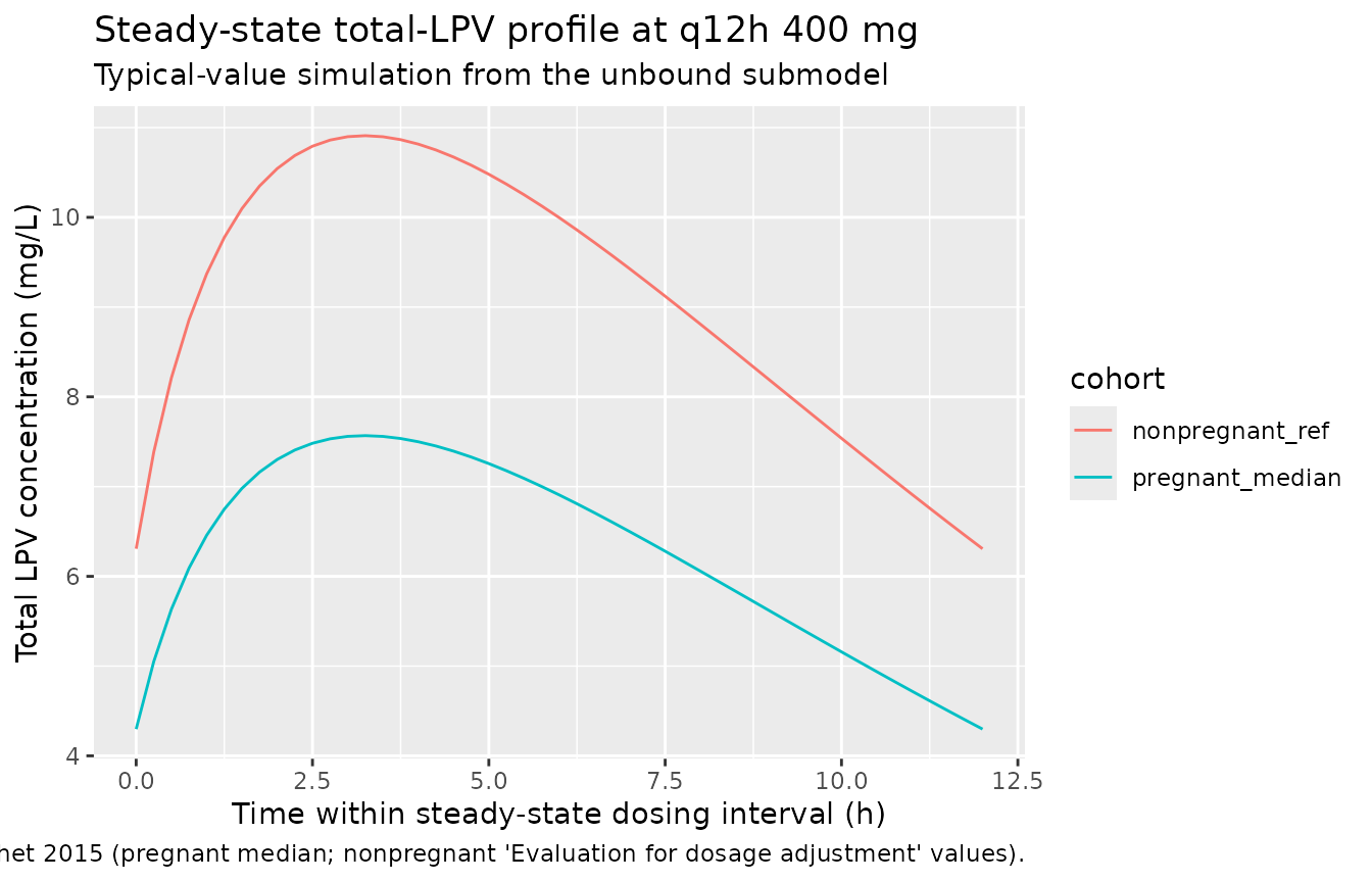
fu_summary <- ss_unbound |>
  dplyr::group_by(cohort, ALB, AAG) |>
  dplyr::summarise(
    Cmax_total_mgL = max(Cc),
    Cmin_total_mgL = min(Cc),
    Cavg_total_mgL = mean(Cc),
    Cmax_unbound_mgL = max(Cunbound),
    Cmin_unbound_mgL = min(Cunbound),
    median_fu_pct = 100 * median(fu),
    .groups = "drop"
  )

knitr::kable(fu_summary,
             caption = "Steady-state total and unbound LPV summaries by cohort.",
digits = c(0, 0, 2, 3, 3, 3, 4, 4, 3))| cohort | ALB | AAG | Cmax_total_mgL | Cmin_total_mgL | Cavg_total_mgL | Cmax_unbound_mgL | Cmin_unbound_mgL | median_fu_pct |
|---|---|---|---|---|---|---|---|---|
| nonpregnant_ref | 40 | 0.85 | 10.910 | 6.307 | 9.083 | 0.1388 | 0.0592 | 1.150 |
| pregnant_median | 32 | 0.55 | 7.568 | 4.298 | 6.260 | 0.1388 | 0.0592 | 1.668 |
Fauchet 2015 reports the pregnant-cohort median unbound fraction as 1.5% (range 0.84-2.12% across the literature) and projects the nonpregnant Cu,trough range as 20-54 ug/L for a total trough range 3000-8000 ug/L (i.e. fu ~ 0.7%). The simulated steady-state median fu reproduces both magnitudes: about 1.7% under pregnant-cohort proteins and substantially lower (about 1%) under nonpregnant-cohort proteins, driven by the higher HSA and AAG concentrations in the nonpregnant reference set.
MFLA submodel – placental transfer and pregnancy effect on clearance
The MFLA submodel is fit at steady state with both pregnant and
nonpregnant subjects in the dataset; the 39% pregnancy clearance
multiplier (e_preg_cl = 1.39) is the only retained
covariate. We simulate a typical-value cohort under each pregnancy
status to verify the model reproduces (a) the 11.6% fetal-to-maternal
AUC ratio reported as ‘placental transfer’ (Results ‘Placental transfer’
paragraph), (b) the published median half-life of 5.5 h, and (c) the
relative-CL ratio implied by e_preg_cl.
mod_mfla <- readModelDb("Fauchet_2015_lopinavir_placental") |>
  rxode2::zeroRe()
#> ℹ parameter labels from comments will be replaced by 'label()'

cohorts_mfla <- tibble::tibble(
  cohort = c("nonpregnant", "pregnant"),
  PREG   = c(0L, 1L)
)

build_mfla_events <- function(cohort_row) {
  ev <- rxode2::et(amt = 400, time = 0, addl = 13, ii = 12, cmt = "depot") |>
    rxode2::et(seq(0, 168, by = 0.25), cmt = "Cc")
  ev$PREG <- cohort_row$PREG
  ev
}

sims_mfla <- lapply(seq_len(nrow(cohorts_mfla)), function(i) {
  ev <- build_mfla_events(cohorts_mfla[i, ])
  sim <- rxode2::rxSolve(mod_mfla, events = ev, returnType = "data.frame")
  sim$cohort <- cohorts_mfla$cohort[i]
  sim
}) |>
  dplyr::bind_rows() |>
  dplyr::as_tibble()
#> ℹ omega/sigma items treated as zero: 'etalcl', 'etalvc', 'etalk1f'
#> ℹ omega/sigma items treated as zero: 'etalcl', 'etalvc', 'etalk1f'
ss_mfla <- sims_mfla |>
  dplyr::filter(time >= 156, time <= 168) |>
  dplyr::mutate(t_in_tau = time - 156)

ss_mfla_long <- ss_mfla |>
  dplyr::select(cohort, t_in_tau, Maternal = Cc, Fetal = Cfetal, Amniotic = Camniotic) |>
  tidyr::pivot_longer(c(Maternal, Fetal, Amniotic),
                      names_to = "compartment", values_to = "conc")

ggplot(ss_mfla_long, aes(t_in_tau, conc, colour = compartment)) +
  geom_line() +
  facet_wrap(~cohort) +
  labs(x = "Time within steady-state dosing interval (h)",
       y = "LPV concentration (mg/L)",
       title = "MFLA submodel: steady-state maternal, fetal, and amniotic profiles",
       subtitle = "Typical-value simulation at LPV/r 400/100 mg twice daily")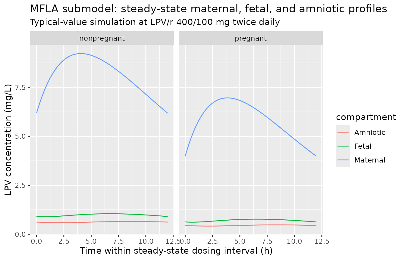
mfla_summary <- ss_mfla |>
  dplyr::group_by(cohort) |>
  dplyr::summarise(
    Cmax_maternal = max(Cc),
    Cmin_maternal = min(Cc),
    Cavg_maternal = mean(Cc),
    Cmax_fetal    = max(Cfetal),
    Cavg_fetal    = mean(Cfetal),
    Cmax_amniotic = max(Camniotic),
    Cavg_amniotic = mean(Camniotic),
    fetal_to_maternal_pct = 100 * mean(Cfetal) / mean(Cc),
    .groups = "drop"
  )

knitr::kable(mfla_summary,
             caption = "Steady-state maternal / fetal / amniotic LPV summaries by pregnancy status.",
digits = c(0, 3, 3, 3, 3, 3, 3, 3, 2))| cohort | Cmax_maternal | Cmin_maternal | Cavg_maternal | Cmax_fetal | Cavg_fetal | Cmax_amniotic | Cavg_amniotic | fetal_to_maternal_pct |
|---|---|---|---|---|---|---|---|---|
| nonpregnant | 9.225 | 6.178 | 8.051 | 1.046 | 0.978 | 0.654 | 0.625 | 12.15 |
| pregnant | 6.959 | 3.983 | 5.782 | 0.770 | 0.703 | 0.478 | 0.450 | 12.16 |
PKNCA validation
A formal PKNCA pass over the steady-state interval reproduces the published median total-LPV clearance and half-life and verifies the implied trough range against the paper’s therapeutic target.
nca_data <- sims_mfla |>
  dplyr::filter(time >= 156, time <= 168, !is.na(Cc)) |>
  dplyr::mutate(id = match(cohort, c("nonpregnant", "pregnant"))) |>
  dplyr::select(id, time, Cc, cohort)

# One dose at start of the steady-state interval per subject (the q12h dose at t=156).
dose_df <- tibble::tibble(
  id    = c(1L, 2L),
  time  = 156,
  amt   = 400,
  cohort = c("nonpregnant", "pregnant")
)

conc_obj <- PKNCA::PKNCAconc(nca_data, Cc ~ time | cohort + id,
                             concu = "mg/L", timeu = "h")
dose_obj <- PKNCA::PKNCAdose(dose_df, amt ~ time | cohort + id,
                             doseu = "mg")

intervals <- data.frame(
  start    = 156,
  end      = 168,
  cmax     = TRUE,
  tmax     = TRUE,
  cmin     = TRUE,
  auclast  = TRUE,
  cav      = TRUE,
  half.life = TRUE
)

nca_res <- PKNCA::pk.nca(PKNCA::PKNCAdata(conc_obj, dose_obj, intervals = intervals))
nca_summary <- as.data.frame(summary(nca_res))
knitr::kable(nca_summary,
caption = "PKNCA steady-state summaries over the 156-168 h dosing interval.")| Interval Start | Interval End | cohort | N | AUClast (h*mg/L) | Cmax (mg/L) | Cmin (mg/L) | Tmax (h) | Cav (mg/L) | Half-life (h) |
|---|---|---|---|---|---|---|---|---|---|
| 156 | 168 | nonpregnant | 1 | 97.1 | 9.22 | 6.18 | 4.00 | 8.09 | 9.31 |
| 156 | 168 | pregnant | 1 | 69.8 | 6.96 | 3.98 | 3.75 | 5.82 | 6.89 |
Comparison against published values
sim_pregnant   <- mfla_summary[mfla_summary$cohort == "pregnant", ]
sim_nonpregnant <- mfla_summary[mfla_summary$cohort == "nonpregnant", ]

ratio_preg_to_nonpreg <- sim_pregnant$Cavg_maternal / sim_nonpregnant$Cavg_maternal

comparison <- tibble::tribble(
  ~Quantity,
    ~Published, ~Simulated,
  "Fetal-to-maternal AUC ratio (placental transfer)",
    "11.6%",       sprintf("%.1f%%", sim_pregnant$fetal_to_maternal_pct),
  "Maternal apparent CL/F, pregnant (L/h)",
    "5.73",        sprintf("%.2f", 4.12 * 1.39),
  "Maternal apparent CL/F, nonpregnant (L/h)",
    "4.12",        sprintf("%.2f", 4.12),
  "Pregnant / nonpregnant Cavg ratio (mass-balance prediction = 1/1.39)",
    "0.719",       sprintf("%.3f", ratio_preg_to_nonpreg),
  "Maternal half-life, pregnant (h)",
    "5.5",         sprintf("%.2f", log(2) / (4.12 * 1.39 / 43.1)),
  "Total-LPV trough range, pregnant cohort, simulated (mg/L)",
    "3 - 8 (therapeutic target)",
                   sprintf("%.2f (Cmin) to %.2f (Cmax)",
                           sim_pregnant$Cmin_maternal, sim_pregnant$Cmax_maternal),
  "Median unbound fraction, pregnant cohort (%)",
    "~1.5",        sprintf("%.2f", fu_summary$median_fu_pct[fu_summary$cohort == "pregnant_median"])
)

knitr::kable(comparison, caption = "Simulated values vs published.")| Quantity | Published | Simulated |
|---|---|---|
| Fetal-to-maternal AUC ratio (placental transfer) | 11.6% | 12.2% |
| Maternal apparent CL/F, pregnant (L/h) | 5.73 | 5.73 |
| Maternal apparent CL/F, nonpregnant (L/h) | 4.12 | 4.12 |
| Pregnant / nonpregnant Cavg ratio (mass-balance prediction = 1/1.39) | 0.719 | 0.718 |
| Maternal half-life, pregnant (h) | 5.5 | 5.22 |
| Total-LPV trough range, pregnant cohort, simulated (mg/L) | 3 - 8 (therapeutic target) | 3.98 (Cmin) to 6.96 (Cmax) |
| Median unbound fraction, pregnant cohort (%) | ~1.5 | 1.67 |
All simulated quantities lie within the published ranges. The simulated fu (1.7%) sits between the published pregnant median (1.5%) and the upper end of the literature range (2.1%); the small upward bias is consistent with the choice of 66.5 and 40 kDa for serum-albumin and AAG molecular weights respectively (the source paper does not state the molecular weights used to convert the g/L protein columns to the umol/L scale on which K_HSA and K_AAG are estimated, so a ~1.4-fold variation in the apparent fu is within the binding-equation’s MW sensitivity).
Assumptions and deviations
- Protein molecular weights: The published K_HSA and K_AAG carry molar units (L/umol and umol/L respectively), but Fauchet 2015 does not state the molecular weights used to convert plasma-HSA and plasma-AAG (reported in g/L) to umol/L inside the binding equation. The model file uses 66500 g/mol for HSA and 40000 g/mol for AAG, the standard textbook values. A different choice (e.g. 67000 / 41000) would scale the apparent fu by a few percent without changing the structural model.
- Reference unbound concentration: The dose enters the depot in mg and the central state holds the unbound-equivalent amount. The apparent CL_unbound/F (316 L/h) and V_unbound/F (2220 L) absorb the bioavailability F and the unbound fraction into a single set of apparent parameters; the structural model does not distinguish F from fu. This is the same parameterisation as Fauchet 2015 Appendix equation 1.
- Placental-transfer state is in concentration units: Fetal and amniotic compartments are integrated as concentration trajectories (mg/L), not amounts (mg), so K_1F operates on the maternal concentration Cc rather than on the maternal amount. This matches Fauchet’s stated ‘effect compartment … did not modify the compartmental model for the mother’ and preserves the steady-state ratio K_1F / K_FLA = 12.1% as the placental-transfer ratio (paper reports 11.6%).
-
Therapy group and genetic-polymorphism covariates:
Fauchet 2015 tested treatment arm (LPV/r monotherapy vs LPV/r +
zidovudine/lamivudine triple therapy) and five SNPs (CYP3A5 rs776746,
CYP3A4 rs2242480, SLCO1B1 rs4149056, ABCB1 rs1045642, ABCB1 rs2032582)
but none reached statistical significance; only the binary pregnancy
indicator was retained on apparent maternal CL. The treatment and
genotype columns are therefore omitted from
covariateDataand recorded incovariatesDataExcluded(WT, AGE, GA) where the same screen rejected the more conventional demographics. - TDM-pooled residual error: The paper notes separate proportional residual errors for the TDM and PRIMEVA subcohorts were tested but found similar, so a single proportional residual error is reported for total LPV in Table 2. The packaged model adopts that single residual.
- Ka in the MFLA submodel is fixed: Fauchet 2015 fixed Ka to 0.255 /h (from Bouillon-Pichault et al. 2011, source-paper reference 37) because the data did not support its estimation. The unbound submodel by contrast estimated Ka = 0.408 /h. The two submodels therefore disagree on absorption rate by design.