Bedaquiline (Kurosawa 2021)
Source:vignettes/articles/Kurosawa_2021_bedaquiline.Rmd
Kurosawa_2021_bedaquiline.RmdModel and source
- Citation: Kurosawa K, Rossenu S, Biewenga J, Ouwerkerk-Mahadevan S, Willems W, Ernault E, Kambili C (2021). Population Pharmacokinetic Analysis of Bedaquiline-Clarithromycin for Dose Selection Against Pulmonary Nontuberculous Mycobacteria Based on a Phase 1, Randomized, Pharmacokinetic Study. Journal of Clinical Pharmacology 61(10):1344-1355. doi:10.1002/jcph.1887. All parameters other than the clarithromycin effect are fixed to the previously developed model reprinted in Kurosawa 2021 Supplemental Table S1: McLeay SC, Vis P, van Heeswijk RPG, Green B (2014). Population pharmacokinetics of bedaquiline (TMC207), a novel antituberculosis drug. Antimicrobial Agents and Chemotherapy 58(9):5315-5324. doi:10.1128/AAC.01418-13 (structure from McLeay 2014 Fig. 1 and Results; values cross-checked against McLeay 2014 Table 3).
- Description: Four-compartment population PK model for oral bedaquiline with the dual zero-order absorption input of McLeay 2014, updated by Kurosawa 2021 with the effect of steady-state clarithromycin (500 mg every 12 hours) on bedaquiline apparent clearance, estimated from a phase 1 crossover study in 16 healthy adults (NCT03800550). A fraction FR1 of each dose enters a depot as a zero-order input over DUR1 after a formulation-dependent lag Tlag and passes to the central compartment at a fixed rate of 1,000 1/h; the remaining 1 - FR1 enters the central compartment directly as a zero-order input over DUR2 after a lag of Tlag + Tlag,add. Every structural, covariate, variability and residual parameter is fixed to the McLeay 2014 final estimates (study on relative bioavailability, Black race and healthy-volunteer / drug-sensitive-TB status on CL/F, female sex on Vc/F); only the clarithromycin effect was estimated, CL/F x (1 - 0.37) with clarithromycin co-administration.
- Article: https://doi.org/10.1002/jcph.1887 (open access, PMC8518967)
- Previously developed model: McLeay et al. 2014, https://doi.org/10.1128/AAC.01418-13
Kurosawa 2021 ran a phase 1 crossover study (NCT03800550) of a single 100 mg bedaquiline tablet given alone (treatment A) or on day 5 of clarithromycin 500 mg every 12 hours (treatment B). The population PK analysis took the four-compartment bedaquiline model of McLeay 2014, confirmed that it described the monotherapy data, and then estimated a single new parameter: the effect of clarithromycin on bedaquiline apparent clearance,
a 37% reduction. Every other parameter was carried unchanged from
McLeay 2014 (Kurosawa 2021 Supplemental Table S1, whose “updated model”
column is blank for everything except the clarithromycin effect), and is
therefore fixed() in the packaged model. The updated model
was then used to simulate 48-week bedaquiline regimens with
clarithromycin for pulmonary nontuberculous mycobacterial disease.
Population
The updated model was estimated on 16 healthy White adults in Belgium (9 women, 7 men), median age 43 years (24-55), median weight 65.65 kg (56.8-100.0) and median BMI 22.44 kg/m^2 (18.9-29.5) (Kurosawa 2021 Table 1). The fixed parameters come from McLeay 2014: 5,222 concentrations from 480 subjects (111 healthy volunteers, 44 patients with drug-sensitive TB and 325 patients with MDR-TB) in nine phase I/II studies.
str(readModelDb("Kurosawa_2021_bedaquiline")()$population)
#> List of 12
#>  $ species       : chr "human"
#>  $ n_subjects    : int 16
#>  $ n_studies     : int 1
#>  $ age_range     : chr "24-55 years (median 43)"
#>  $ weight_range  : chr "56.8-100.0 kg (median 65.65)"
#>  $ bmi_range     : chr "18.9-29.5 kg/m^2 (median 22.44)"
#>  $ sex_female_pct: num 56.3
#>  $ race_ethnicity: Named num 100
#>   ..- attr(*, "names")= chr "White"
#>  $ disease_state : chr "Healthy adults"
#>  $ dose_range    : chr "Single oral 100 mg bedaquiline tablet with a standardized breakfast, alone (treatment A) or on day 5 of clarith"| __truncated__
#>  $ regions       : chr "Belgium (single centre), March-June 2019"
#>  $ notes         : chr "Kurosawa 2021 Table 1. Only the clarithromycin effect was estimated on these 16 subjects; every other parameter"| __truncated__
Source trace
Every value is also traced in a comment beside its ini()
line in
inst/modeldb/specificDrugs/Kurosawa_2021_bedaquiline.R.
“S1” is Kurosawa 2021 Supplemental Table S1 (which reprints the McLeay
2014 Table 3 estimates in its “previously developed model” column).
| Equation / parameter | Value | Source location |
|---|---|---|
lcl (CL/F, reference individual) |
2.78 L/h, fixed | S1; McLeay 2014 Table 3 |
lvc (Vc/F) |
164 L, fixed | S1 |
lq, lvp (CLp1/F, Vp1/F) |
11.8 L/h, 178 L, fixed | S1 |
lq2, lvp2 (CLp2/F, Vp2/F) |
8.03 L/h, 3010 L, fixed | S1 |
lq3, lvp3 (CLp3/F, Vp3/F) |
3.58 L/h, 7350 L, fixed | S1 |
lka (input compartment to central) |
1000 1/h, fixed | McLeay 2014 Results and Fig. 1 |
logitfrel (FR1, fraction into the depot arm) |
58.5%, fixed | S1; logit constraint, McLeay 2014 Results |
ld1, ld2 (DUR1, DUR2) |
2.22 h, 1.48 h, fixed | S1 ‘D1’, ‘D2’ |
ltlag, ltlag_tablet (Tlag) |
0.541 h solution, 0.917 h tablet, fixed | S1 ‘ALAG1 solution’, ‘ALAG1 tablet’ |
ltlag_add (Tlag,add) |
1.48 h, fixed | S1 ‘TLAG’ |
| lag of the central arm | Tlag + Tlag,add | McLeay 2014 Fig. 1 |
lfdepot (F, studies C208 / C209) |
1, fixed reference | McLeay 2014 Results |
e_study_bdq_cde102_c104_f |
1.51, fixed | S1 |
e_study_other_f |
2.03, fixed | S1 ‘Other studies on F’ |
e_race_black_cl |
+52.0%, fixed | S1 |
e_nonmdr_cl (healthy volunteers / DS-TB) |
+37.5%, fixed | S1 |
e_sexf_vc |
-15.7%, fixed | S1 |
e_conmed_clarithromycin_cl |
-0.37 (RSE 11%), estimated | S1 ‘Effect CLR on CL/F’; Results |
Covariate form (1 + theta)^cov
|
n/a | Kurosawa 2021 Methods equation; McLeay 2014 equation 5 |
etalcl, etalvc
|
0.504^2, 0.391^2, correlation 0.407 | S1 ‘BSV’ column and ‘Correlation CL/Vc’ |
etalogitfrel |
1.13^2 (logit scale) | S1 ‘BSV’ FR1 = 113 |
etalfdepot |
0.396^2 | S1 ‘Between-subject variability on F’ |
expSd, expSdC208C209
|
0.206, 0.277 | S1 ‘RUV’ rows; log-transform-both-sides, McLeay 2014 equation 2 |
d/dt() system |
n/a | McLeay 2014 Fig. 1 (four compartments, dual zero-order input) |
Dual zero-order absorption
Each oral dose is split: a fraction FR1 = 58.5% enters an input
compartment as a zero-order infusion over DUR1 = 2.22 h, starting after
the lag Tlag, and is passed to the central compartment at 1,000 1/h (so
this arm is effectively zero-order too); the remaining 41.5% enters the
central compartment directly as a zero-order infusion over DUR2 = 1.48
h, starting after Tlag + Tlag,add. Every administration is therefore
two dose records at the same time, one to
depot and one to central, each carrying the
whole dose amount (the f() terms perform the split) and its
zero-order duration.
The durations are passed explicitly in a dur column.
They are fixed constants with no random effect, so this is numerically
the same as requesting the modelled durations with
rate = -2, and it avoids a failure of some rxode2 releases
to solve two simultaneous modelled-duration doses into different
compartments.
mod <- readModelDb("Kurosawa_2021_bedaquiline")
ui <- rxode2::rxode2(mod)
#> ℹ parameter labels from comments will be replaced by 'label()'
modTyp <- rxode2::zeroRe(ui)
#> Warning: No sigma parameters in the model

DUR1 <- 2.22 # S1 'D1', fixed
DUR2 <- 1.48 # S1 'D2', fixed

# One row per subject per dose time and arm; `id` and covariates are added
# by the caller.
doseRows <- function(times, amt) {
  dplyr::bind_rows(
    tibble(time = times, amt = amt, cmt = "depot", evid = 1L, dur = DUR1),
    tibble(time = times, amt = amt, cmt = "central", evid = 1L, dur = DUR2)
  )
}
# Observation rows target the ODE state `central`; rxode2 returns Cc.
obsRows <- function(times) {
  tibble(time = times, amt = NA_real_, cmt = "central", evid = 0L, dur = NA_real_)
}

# Covariates of the Kurosawa 2021 healthy volunteers: 100 mg tablet, not
# MDR-TB (so CL/F carries the +37.5% healthy-volunteer effect), a new study
# (so relative F is the 'other studies' 2.03), all White.
addHvCov <- function(d) {
  dplyr::mutate(d,
    RACE_BLACK = 0L, DIS_TB_MDR = 0L, STUDY_BDQ_C208_C209 = 0L,
    STUDY_BDQ_CDE102_C104 = 0L, FORM_TABLET = 1L
  )
}
evTyp <- dplyr::bind_rows(doseRows(0, 100), obsRows(seq(0, 12, by = 0.02))) |>
  dplyr::arrange(time, dplyr::desc(evid)) |>
  dplyr::mutate(id = 1L, SEXF = 0L, CONMED_CLARITHROMYCIN = 0L) |>
  addHvCov()
simTyp <- rxode2::rxSolve(modTyp, evTyp, returnType = "data.frame",
                          rtol = 1e-10, atol = 1e-12)
#> ℹ omega/sigma items treated as zero: 'etalcl', 'etalvc', 'etalogitfrel', 'etalfdepot'

ggplot(simTyp, aes(time, Cc * 1000)) +
  geom_line() +
  geom_vline(xintercept = c(0.917, 0.917 + 2.22), linetype = "dashed", colour = "grey40") +
  geom_vline(xintercept = c(0.917 + 1.48, 0.917 + 1.48 + 1.48), linetype = "dotted", colour = "grey40") +
  labs(x = "Time after dose (h)", y = "Bedaquiline (ng/mL)",
       caption = "Dashed: depot arm (Tlag to Tlag + DUR1). Dotted: direct central arm (Tlag + Tlag,add to + DUR2).")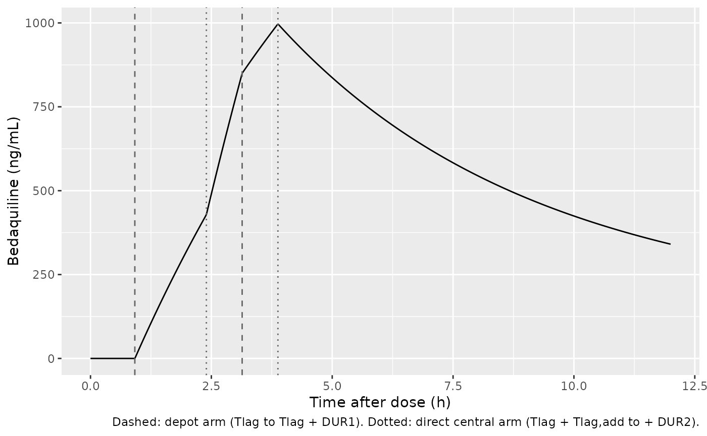
Typical 100 mg tablet profile in a healthy male volunteer over the first 12 h, and the two input arms.
# Nothing enters before the tablet lag of 0.917 h. Relative floor: the ODE
# path can undershoot zero by about atol.
preLag <- simTyp$Cc[simTyp$time < 0.9]
stopifnot(all(abs(preLag) < 1e-6 * max(simTyp$Cc)))
stopifnot(max(simTyp$Cc[simTyp$time > 1]) > 0)
Structural gates
Two closed-form identities check the dose split and the
clarithromycin effect independently of any published number. For a
single dose the whole bioavailable amount is eventually cleared, so
CL * AUC(0-inf) = F * Dose whatever FR1, the durations and
the lags are; a missing dose record, a split that does not sum to one,
or a bioavailability applied to one arm only would break it. And the
clarithromycin factor on the individual clearance must be exactly
1 - 0.37.
# Terminal half-life is several months, so integrate on a log-spaced grid
# out to about 11 years and close the remainder analytically from the last
# log-linear slope.
tLong <- sort(unique(c(seq(0, 12, by = 0.01), exp(seq(log(12), log(1e5), length.out = 3000)))))
evLong <- dplyr::bind_rows(doseRows(0, 100), obsRows(tLong)) |>
  dplyr::arrange(time, dplyr::desc(evid)) |>
  dplyr::mutate(id = 1L, SEXF = 0L) |>
  addHvCov()
auc_check <- lapply(0:1, function(clr) {
  s <- rxode2::rxSolve(modTyp, dplyr::mutate(evLong, CONMED_CLARITHROMYCIN = clr),
                       returnType = "data.frame", rtol = 1e-10, atol = 1e-14,
                       maxsteps = 1e6)
  auc <- sum(diff(s$time) * (head(s$Cc, -1) + tail(s$Cc, -1)) / 2)
  n <- nrow(s)
  lz <- -diff(log(s$Cc[(n - 1):n])) / diff(s$time[(n - 1):n])
  tibble(CONMED_CLARITHROMYCIN = clr, cl = s$cl[1], fbio = s$fbio[1],
         auc_inf = auc + s$Cc[n] / lz)
}) |> dplyr::bind_rows() |>
  dplyr::mutate(ratio = cl * auc_inf / (fbio * 100))
#> ℹ omega/sigma items treated as zero: 'etalcl', 'etalvc', 'etalogitfrel', 'etalfdepot'
#> ℹ omega/sigma items treated as zero: 'etalcl', 'etalvc', 'etalogitfrel', 'etalfdepot'
knitr::kable(auc_check, digits = 5,
caption = "CL x AUC(0-inf) / (F x Dose); the identity requires 1.")| CONMED_CLARITHROMYCIN | cl | fbio | auc_inf | ratio |
|---|---|---|---|---|
| 0 | 3.82250 | 2.03 | 53.10669 | 1 |
| 1 | 2.40818 | 2.03 | 84.29633 | 1 |
Single-dose crossover study (Kurosawa 2021 Tables 2 and 3, Figure 2)
The virtual cohort mirrors the study: healthy White adults given one 100 mg tablet alone (A) or with steady-state clarithromycin (B), sampled to 240 h. To make the two arms a true crossover, the same 200 subjects receive both treatments: their random effects are drawn once in R from the model’s omega matrix and supplied as data to the typical-value model. This also makes the cohort, and every assertion below, identical on every machine, because it does not depend on rxode2’s per-thread random-number streams.
set.seed(20210801)
omega <- ui$omega
omega <- matrix(as.numeric(omega), nrow(omega), dimnames = dimnames(omega))
drawEtas <- function(n, omega) {
  z <- matrix(stats::rnorm(n * nrow(omega)), n)
  e <- z %*% chol(omega)
  colnames(e) <- rownames(omega)
  tibble::as_tibble(e) |> dplyr::mutate(id = seq_len(n), .before = 1)
}
nSD <- 200L
etasSD <- drawEtas(nSD, omega)
sexSD <- tibble(id = seq_len(nSD), SEXF = stats::rbinom(nSD, 1, 9 / 16))

tSD <- sort(unique(c(0, 0.5, seq(1, 8, by = 0.25), 12, 24, 36, 48, 72, 96, 120, 168, 240)))
evSD <- lapply(c(A = 0L, B = 1L), function(clr) {
  one <- dplyr::bind_rows(doseRows(0, 100), obsRows(tSD)) |>
    dplyr::arrange(time, dplyr::desc(evid))
  tidyr::crossing(sexSD, one) |>
    dplyr::arrange(id, time, dplyr::desc(evid)) |>
    dplyr::mutate(CONMED_CLARITHROMYCIN = clr) |>
    addHvCov()
})

simSD <- lapply(names(evSD), function(trt) {
  rxode2::rxSolve(modTyp, evSD[[trt]], params = etasSD, returnType = "data.frame") |>
    dplyr::mutate(treatment = trt)
}) |> dplyr::bind_rows()
#> Warning: multi-subject simulation without without 'omega'
#> Warning: multi-subject simulation without without 'omega'
simSD |>
  dplyr::group_by(treatment, time) |>
  dplyr::summarise(mean = mean(Cc * 1000), sd = sd(Cc * 1000), .groups = "drop") |>
  dplyr::mutate(treatment = ifelse(treatment == "A", "A: bedaquiline alone",
                                   "B: with clarithromycin")) |>
  ggplot(aes(time, mean, colour = treatment)) +
  geom_line() +
  geom_errorbar(aes(ymin = pmax(mean - sd, 0), ymax = mean + sd), width = 3, alpha = 0.5) +
  labs(x = "Time after bedaquiline dose (h)", y = "Bedaquiline (ng/mL)", colour = NULL,
       caption = "Simulated, 200 virtual subjects per treatment (paired).") +
  theme(legend.position = "bottom")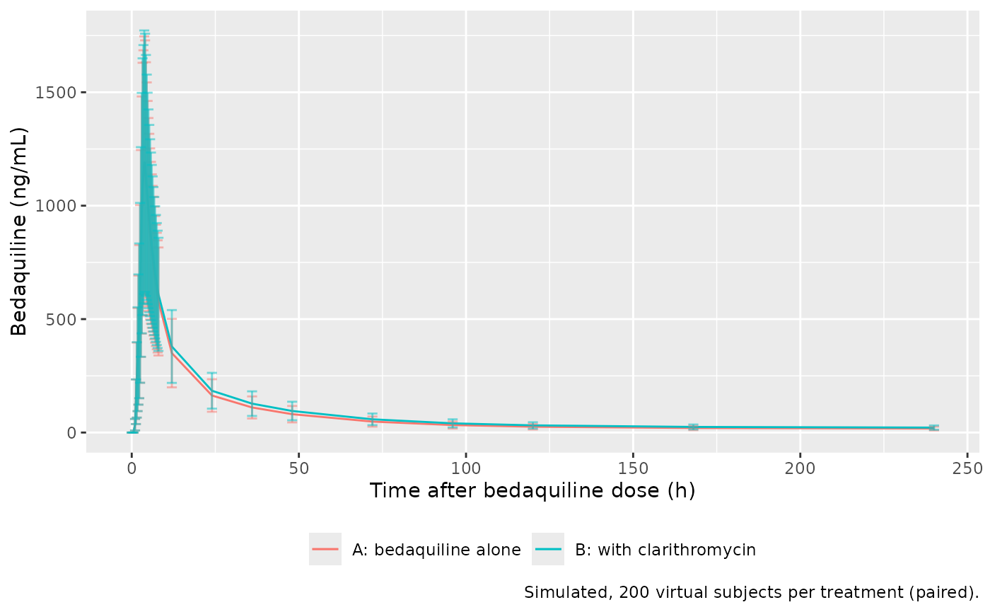
Replicates Figure 2A of Kurosawa 2021: mean (SD) bedaquiline concentration after a single 100 mg tablet, with and without clarithromycin.
PKNCA
concSD <- simSD |>
  dplyr::filter(!is.na(Cc)) |>
  dplyr::mutate(Cc = Cc * 1000) |>
  dplyr::select(id, time, Cc, treatment)
doseSD <- concSD |> dplyr::distinct(id, treatment) |> dplyr::mutate(time = 0, amt = 100)
intervalsSD <- data.frame(
  start = 0, end = c(72, 240),
  cmax = c(TRUE, FALSE), tmax = c(TRUE, FALSE), auclast = TRUE
)
ncaSD <- PKNCA::pk.nca(PKNCA::PKNCAdata(
  PKNCA::PKNCAconc(concSD, Cc ~ time | treatment + id),
  PKNCA::PKNCAdose(doseSD, amt ~ time | treatment + id),
  intervals = intervalsSD
))
resSD <- as.data.frame(ncaSD) |>
  dplyr::mutate(PPTESTCD = dplyr::case_when(
    PPTESTCD == "auclast" & end == 72 ~ "auc72",
    PPTESTCD == "auclast" & end == 240 ~ "auc240",
    TRUE ~ PPTESTCD
  ))

# Geometric means of the simulated subjects (Table 3 reports geometric means).
simGM <- resSD |>
  dplyr::filter(PPTESTCD %in% c("cmax", "auc72", "auc240")) |>
  dplyr::group_by(treatment, PPTESTCD) |>
  dplyr::summarise(PPORRES = exp(mean(log(PPORRES))), .groups = "drop") |>
  dplyr::bind_rows(
    resSD |> dplyr::filter(PPTESTCD == "tmax") |>
      dplyr::group_by(treatment, PPTESTCD) |>
      dplyr::summarise(PPORRES = median(PPORRES), .groups = "drop")
  )

# Kurosawa 2021 Table 3 geometric means (n = 16, both periods) and Table 2
# median tmax (period 1).
published <- tibble::tribble(
  ~treatment, ~cmax, ~tmax, ~auc72, ~auc240,
  "A",        1277,  5.00,  13831,  18482,
  "B",        1285,  5.00,  15458,  21065
)
cmpSD <- nlmixr2lib::ncaComparisonTable(
  simulated = simGM, reference = published, by = "treatment",
  params = c("cmax", "tmax", "auc72", "auc240"),
  units = c(cmax = "ng/mL", tmax = "h", auc72 = "ng*h/mL", auc240 = "ng*h/mL"),
  tolerance_pct = 20
)
#> Warning: ncaParamLabel(): unknown PKNCA code(s) returned as-is: 'auc72',
#> 'auc240'
knitr::kable(cmpSD, caption = paste(
  "Simulated vs published single-dose NCA (A: bedaquiline alone; B: with",
  "clarithromycin). Cmax and AUC are geometric means; tmax is the median.",
  "auc72 = AUC(0-72 h), auc240 = AUC(0-240 h).",
  if (!is.null(attr(cmpSD, "footnote"))) attr(cmpSD, "footnote") else ""
))| NCA parameter | treatment | Reference | Simulated | % diff |
|---|---|---|---|---|
| Cmax (ng/mL) | A | 1280 | 1070 | -16.4% |
| Cmax (ng/mL) | B | 1280 | 1080 | -15.8% |
| Tmax (h) | A | 5 | 3.88 | -22.5%* |
| Tmax (h) | B | 5 | 4 | -20.0% |
| auc240 (ng*h/mL) | A | 18500 | 16900 | -8.5% |
| auc240 (ng*h/mL) | B | 21100 | 19000 | -9.6% |
| auc72 (ng*h/mL) | A | 13800 | 13200 | -4.6% |
| auc72 (ng*h/mL) | B | 15500 | 14400 | -6.8% |
gmr <- simGM |>
  dplyr::filter(PPTESTCD %in% c("auc72", "auc240", "cmax")) |>
  tidyr::pivot_wider(names_from = treatment, values_from = PPORRES) |>
  dplyr::mutate(simulated_GMR = B / A,
                published_GMR = c(auc240 = 1.1397, auc72 = 1.1177, cmax = 1.0066)[PPTESTCD])
knitr::kable(gmr, digits = 3,
caption = "Treatment B / A geometric mean ratio (published: Kurosawa 2021 Table 3).")| PPTESTCD | A | B | simulated_GMR | published_GMR |
|---|---|---|---|---|
| auc240 | 16914.703 | 19044.565 | 1.126 | 1.140 |
| auc72 | 13199.379 | 14408.998 | 1.092 | 1.118 |
| cmax | 1068.056 | 1081.592 | 1.013 | 1.007 |
stopifnot(
  # Structural: AUC over 0-240 h sits on the published geometric mean. A
  # mis-scaled F, CL or dose would move it by far more than 20%.
  all(abs(simGM$PPORRES[simGM$PPTESTCD == "auc240"] /
            published$auc240 - 1) < 0.2),
  # Clarithromycin raises AUC(0-240 h) without changing Cmax, as published.
  gmr$simulated_GMR[gmr$PPTESTCD == "auc240"] > 1.03,
  gmr$simulated_GMR[gmr$PPTESTCD == "auc240"] < 1.25,
  abs(gmr$simulated_GMR[gmr$PPTESTCD == "cmax"] - 1) < 0.05
)
Simulated AUC(0-72 h) and AUC(0-240 h) are 5%-10% below the published geometric means, and the clarithromycin ratio for AUC(0-240 h) is 1.13 against the observed 1.14. The published geometric means pool both study periods, and Kurosawa 2021 reports carry-over of the first bedaquiline dose into period 2 (AUC(0-240 h) 8%-18% higher in period 2 than in period 1, Table 2), which a single-dose simulation does not include. Simulated Cmax is about 16% lower than observed and the simulated median tmax is earlier (about 4 h vs 5 h; the starred row); Kurosawa 2021 notes that the updated model had its largest conditional weighted residuals in the absorption phase (1-2 h after dosing). None of these differences is tuned away.
Steady-state regimens (Kurosawa 2021 Table 5 and Figure 3)
Kurosawa 2021 simulated 48 weeks of bedaquiline in non-Black adults (1:1 male:female) with a disease status similar to MDR-TB. The reference regimen is the MDR-TB regimen without clarithromycin (400 mg once daily for 2 weeks, then 200 mg three times a week); regimens A-D add clarithromycin:
- A: 400 mg once daily for 2 weeks, then 200 mg twice a week
- B: 400 mg once daily for 2 weeks, then 100 mg three times a week
- C: 400 mg once daily for 2 weeks, then 100 mg twice a week
- D: 400 mg once daily for 2 weeks, then 100 mg five times a week
The simulation below uses the same 200 subjects for every regimen,
tablet formulation, DIS_TB_MDR = 1 (no healthy-volunteer
clearance increase) and the reference-study bioavailability, F =
1 (STUDY_BDQ_C208_C209 = 1). The choice of F is
discussed under Assumptions and deviations: with the 2.03 of
the “other studies” group every simulated exposure is almost exactly
2.03 times Table 5.
set.seed(20210802)
nSS <- 200L
etasSS <- drawEtas(nSS, omega)
sexSS <- tibble(id = seq_len(nSS), SEXF = rep(0:1, length.out = nSS))

# Loading: 400 mg daily on days 0-13. Maintenance from week 3: dose days
# within each week (Monday = 0).
regimens <- tibble(
  regimen = c("MDR-TB (ref.)", "A", "B", "C", "D"),
  maint_amt = c(200, 200, 100, 100, 100),
  days = list(c(0, 2, 4), c(0, 3), c(0, 2, 4), c(0, 3), 0:4),
  clr = c(0L, 1L, 1L, 1L, 1L)
)
tObsSS <- sort(unique(c(
  (1:48) * 168,                    # weekly trough, end of each week
  seq(13 * 24, 14 * 24, by = 0.25), # day 14 (week 2)
  seq(23 * 168, 24 * 168, by = 1), # week 24
  seq(47 * 168, 48 * 168, by = 1)  # week 48
)))
evSS <- lapply(seq_len(nrow(regimens)), function(i) {
  maint <- unlist(lapply(2:47, function(w) (w * 7 + regimens$days[[i]]) * 24))
  one <- dplyr::bind_rows(
    doseRows(c((0:13) * 24, maint), c(rep(400, 14), rep(regimens$maint_amt[i], length(maint)))),
    obsRows(tObsSS)
  ) |> dplyr::arrange(time, dplyr::desc(evid))
  tidyr::crossing(sexSS, one) |>
    dplyr::arrange(id, time, dplyr::desc(evid)) |>
    dplyr::mutate(RACE_BLACK = 0L, DIS_TB_MDR = 1L, STUDY_BDQ_C208_C209 = 1L,
                  STUDY_BDQ_CDE102_C104 = 0L, FORM_TABLET = 1L,
                  CONMED_CLARITHROMYCIN = regimens$clr[i])
})
names(evSS) <- regimens$regimen
simSS <- lapply(names(evSS), function(r) {
  rxode2::rxSolve(modTyp, evSS[[r]], params = etasSS, returnType = "data.frame") |>
    dplyr::mutate(regimen = r)
}) |> dplyr::bind_rows()
#> Warning: multi-subject simulation without without 'omega'
#> Warning: multi-subject simulation without without 'omega'
#> Warning: multi-subject simulation without without 'omega'
#> Warning: multi-subject simulation without without 'omega'
#> Warning: multi-subject simulation without without 'omega'
simSS |>
  dplyr::filter(time %in% ((1:48) * 168)) |>
  dplyr::group_by(regimen, week = time / 168) |>
  dplyr::summarise(ctrough = mean(Cc * 1000), .groups = "drop") |>
  ggplot(aes(week, ctrough, colour = regimen)) +
  geom_line() +
  labs(x = "Week", y = "Mean Ctrough (ng/mL)", colour = NULL,
       caption = "MDR-TB (ref.) is without clarithromycin; A-D are with clarithromycin.")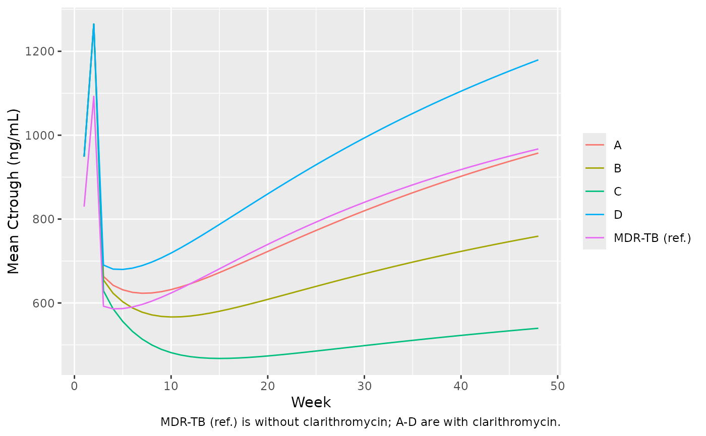
Replicates Figure 3 of Kurosawa 2021: simulated mean bedaquiline trough concentration by week.
PKNCA against Table 5
concSS <- simSS |>
  dplyr::filter(!is.na(Cc), regimen %in% c("MDR-TB (ref.)", "A", "D")) |>
  dplyr::mutate(Cc = Cc * 1000) |>
  dplyr::select(id, time, Cc, regimen)
doseSS <- dplyr::bind_rows(lapply(c("MDR-TB (ref.)", "A", "D"), function(r) {
  evSS[[r]] |> dplyr::filter(evid == 1L, cmt == "depot") |>
    dplyr::select(id, time, amt) |> dplyr::mutate(regimen = r)
}))
# Week 2 = day 14 (AUC0-24); weeks 24 and 48 = AUC over the whole week.
intervalsSS <- data.frame(
  start = c(13 * 24, 23 * 168, 47 * 168),
  end = c(14 * 24, 24 * 168, 48 * 168),
  cmax = TRUE, auclast = TRUE
)
ncaSS <- PKNCA::pk.nca(PKNCA::PKNCAdata(
  PKNCA::PKNCAconc(concSS, Cc ~ time | regimen + id),
  PKNCA::PKNCAdose(doseSS, amt ~ time | regimen + id),
  intervals = intervalsSS
))
simT5 <- as.data.frame(ncaSS) |>
  dplyr::mutate(week = c(`312` = "2", `3864` = "24", `7896` = "48")[as.character(start)]) |>
  dplyr::group_by(regimen, week, PPTESTCD) |>
  dplyr::summarise(PPORRES = mean(PPORRES), .groups = "drop") |>
  # Ctrough is the single concentration at the end of each interval (the
  # next dose starts at that time, after its lag), read directly from the
  # simulation rather than through PKNCA.
  dplyr::bind_rows(
    concSS |>
      dplyr::filter(time %in% c(14 * 24, 24 * 168, 48 * 168)) |>
      dplyr::mutate(week = c(`336` = "2", `4032` = "24", `8064` = "48")[as.character(time)]) |>
      dplyr::group_by(regimen, week) |>
      dplyr::summarise(PPORRES = mean(Cc), .groups = "drop") |>
      dplyr::mutate(PPTESTCD = "ctrough")
  )

# Kurosawa 2021 Table 5, simulated means (n = 1000 per regimen).
table5 <- tibble::tribble(
  ~regimen,        ~week, ~ctrough, ~cmax, ~auclast,
  "MDR-TB (ref.)", "2",   1125,     3274,  42652,
  "MDR-TB (ref.)", "24",  850,      2013,  180526,
  "MDR-TB (ref.)", "48",  1069,     2233,  217615,
  "A",             "2",   1262,     3372,  45900,
  "A",             "24",  794,      1919,  161430,
  "A",             "48",  1009,     2137,  197865,
  "D",             "2",   1258,     3358,  45780,
  "D",             "24",  944,      1596,  191203,
  "D",             "48",  1230,     1884,  239657
)
cmpT5 <- nlmixr2lib::ncaComparisonTable(
  simulated = simT5, reference = table5, by = c("regimen", "week"),
  units = c(ctrough = "ng/mL", cmax = "ng/mL", auclast = "ng*h/mL"),
  tolerance_pct = 20
)
knitr::kable(cmpT5, caption = paste(
  "Simulated vs Kurosawa 2021 Table 5 mean exposures. auclast is AUC(0-24 h)",
  "at week 2 and AUC(0-168 h) at weeks 24 and 48.",
  if (!is.null(attr(cmpT5, "footnote"))) attr(cmpT5, "footnote") else ""
))| NCA parameter | regimen | week | Reference | Simulated | % diff |
|---|---|---|---|---|---|
| Cmax (ng/mL) | MDR-TB (ref.) | 2 | 3270 | 3310 | +1.1% |
| Cmax (ng/mL) | MDR-TB (ref.) | 24 | 2010 | 1960 | -2.6% |
| Cmax (ng/mL) | MDR-TB (ref.) | 48 | 2230 | 2150 | -3.8% |
| Cmax (ng/mL) | A | 2 | 3370 | 3490 | +3.6% |
| Cmax (ng/mL) | A | 24 | 1920 | 1930 | +0.7% |
| Cmax (ng/mL) | A | 48 | 2140 | 2130 | -0.4% |
| Cmax (ng/mL) | D | 2 | 3360 | 3490 | +4.0% |
| Cmax (ng/mL) | D | 24 | 1600 | 1590 | -0.1% |
| Cmax (ng/mL) | D | 48 | 1880 | 1860 | -1.3% |
| AUClast (ng*h/mL) | MDR-TB (ref.) | 2 | 42700 | 40700 | -4.7% |
| AUClast (ng*h/mL) | MDR-TB (ref.) | 24 | 181000 | 167000 | -7.4% |
| AUClast (ng*h/mL) | MDR-TB (ref.) | 48 | 218000 | 199000 | -8.7% |
| AUClast (ng*h/mL) | A | 2 | 45900 | 45100 | -1.7% |
| AUClast (ng*h/mL) | A | 24 | 161000 | 156000 | -3.5% |
| AUClast (ng*h/mL) | A | 48 | 198000 | 189000 | -4.7% |
| AUClast (ng*h/mL) | D | 2 | 45800 | 45100 | -1.4% |
| AUClast (ng*h/mL) | D | 24 | 191000 | 186000 | -2.8% |
| AUClast (ng*h/mL) | D | 48 | 240000 | 231000 | -3.8% |
| Ctrough (ng/mL) | MDR-TB (ref.) | 2 | 1120 | 1090 | -2.9% |
| Ctrough (ng/mL) | MDR-TB (ref.) | 24 | 850 | 783 | -7.9% |
| Ctrough (ng/mL) | MDR-TB (ref.) | 48 | 1070 | 967 | -9.5% |
| Ctrough (ng/mL) | A | 2 | 1260 | 1260 | +0.2% |
| Ctrough (ng/mL) | A | 24 | 794 | 763 | -3.9% |
| Ctrough (ng/mL) | A | 48 | 1010 | 957 | -5.1% |
| Ctrough (ng/mL) | D | 2 | 1260 | 1260 | +0.5% |
| Ctrough (ng/mL) | D | 24 | 944 | 916 | -3.0% |
| Ctrough (ng/mL) | D | 48 | 1230 | 1180 | -4.1% |
pctT5 <- simT5 |>
  dplyr::inner_join(
    tidyr::pivot_longer(table5, c(ctrough, cmax, auclast),
                        names_to = "PPTESTCD", values_to = "ref"),
    by = c("regimen", "week", "PPTESTCD")
  ) |>
  dplyr::mutate(pct = 100 * (PPORRES / ref - 1))
stopifnot(
  nrow(pctT5) == 27L,
  !anyNA(pctT5$pct),
  # Structural: F, CL, the regimen and the clarithromycin effect together
  # put the 27 means on Table 5. With F = 2.03 the median would be +100%.
  abs(median(pctT5$pct)) < 8,
  # Envelope, robust to which subjects land in the tails.
  quantile(abs(pctT5$pct), 0.9) < 15
)
The 27 simulated means match Table 5 closely (median difference -2.9%, largest 9.5% in absolute value), including the week-24 Cmax deficit of regimen D that Kurosawa 2021 singles out.
The between-subject variability scale
Supplemental Table S1 lists the between-subject variability as bare numbers (50.4 for CL/F, 39.1 for Vc/F, 113 for FR1, 39.6 for F) under a “BSV” header, and McLeay 2014 calls them “%CV”. That leaves two readings: the number is the SD of eta (omega = 0.504), or a back-transformed CV (omega^2 = log(1 + 0.504^2)). FR1 carries its eta on the logit scale, where a back-transformed CV has no meaning, which already favours the first. Table 5 supports it: the SD / mean of the simulated trough and AUC depends on the clearance and bioavailability omegas, and the eta-SD reading reproduces the published spread more closely than the log(1 + CV^2) reading, which is too narrow. The same standard-normal draws are used for both readings, so the comparison is paired. (Cmax also depends on the large logit-scale FR1 variance and does not separate the two readings at 200 subjects; in a 1,000-subject check made by the maintainers while building the model, the eta-SD reading was the closer one for all nine Table 5 reference-regimen cells.)
cv <- sqrt(diag(omega))
rho <- omega["etalcl", "etalvc"] / (cv["etalcl"] * cv["etalvc"])
omegaLog <- diag(log(1 + cv^2))
dimnames(omegaLog) <- dimnames(omega)
omegaLog["etalcl", "etalvc"] <- omegaLog["etalvc", "etalcl"] <-
  rho * sqrt(omegaLog["etalcl", "etalcl"] * omegaLog["etalvc", "etalvc"])
# Rescale the SAME eta draws to the alternative omega.
zSS <- as.matrix(etasSS[, rownames(omega)]) %*% solve(chol(omega))
etasLog <- tibble::as_tibble(zSS %*% chol(omegaLog)) |>
  dplyr::mutate(id = etasSS$id, .before = 1)

simLog <- rxode2::rxSolve(modTyp, evSS[["MDR-TB (ref.)"]], params = etasLog,
                          returnType = "data.frame")
#> Warning: multi-subject simulation without without 'omega'
spread <- function(s, reading) {
  wk <- function(lo, hi, lab) s |> dplyr::filter(time >= lo, time <= hi) |>
    dplyr::group_by(id) |>
    dplyr::summarise(ctrough = Cc[which.max(time)], cmax = max(Cc),
                     auc = sum(diff(time) * (head(Cc, -1) + tail(Cc, -1)) / 2)) |>
    dplyr::summarise(dplyr::across(c(ctrough, cmax, auc), ~ sd(.x) / mean(.x))) |>
    dplyr::mutate(week = lab)
  dplyr::bind_rows(wk(312, 336, "2"), wk(3864, 4032, "24"), wk(7896, 8064, "48")) |>
    dplyr::mutate(reading = reading)
}
spreadTab <- dplyr::bind_rows(
  spread(dplyr::filter(simSS, regimen == "MDR-TB (ref.)"), "omega = BSV/100 (packaged)"),
  spread(simLog, "omega^2 = log(1 + CV^2)"),
  tibble(ctrough = c(523 / 1125, 489 / 850, 667 / 1069),
         cmax = c(1657 / 3274, 1059 / 2013, 1212 / 2233),
         auc = c(19684 / 42652, 96964 / 180526, 126252 / 217615),
         week = c("2", "24", "48"), reading = "Kurosawa 2021 Table 5")
)
knitr::kable(spreadTab, digits = 3,
caption = "SD / mean of the MDR-TB reference-regimen exposures.")| ctrough | cmax | auc | week | reading |
|---|---|---|---|---|
| 0.455 | 0.551 | 0.450 | 2 | omega = BSV/100 (packaged) |
| 0.544 | 0.554 | 0.511 | 24 | omega = BSV/100 (packaged) |
| 0.580 | 0.556 | 0.541 | 48 | omega = BSV/100 (packaged) |
| 0.436 | 0.521 | 0.430 | 2 | omega^2 = log(1 + CV^2) |
| 0.520 | 0.525 | 0.489 | 24 | omega^2 = log(1 + CV^2) |
| 0.554 | 0.528 | 0.518 | 48 | omega^2 = log(1 + CV^2) |
| 0.465 | 0.506 | 0.462 | 2 | Kurosawa 2021 Table 5 |
| 0.575 | 0.526 | 0.537 | 24 | Kurosawa 2021 Table 5 |
| 0.624 | 0.543 | 0.580 | 48 | Kurosawa 2021 Table 5 |
gap <- spreadTab |>
  tidyr::pivot_longer(c(ctrough, cmax, auc)) |>
  tidyr::pivot_wider(names_from = reading, values_from = value) |>
  dplyr::mutate(
    sdReading = abs(`omega = BSV/100 (packaged)` - `Kurosawa 2021 Table 5`),
    logReading = abs(`omega^2 = log(1 + CV^2)` - `Kurosawa 2021 Table 5`)
  )
# Trough and AUC: the packaged reading is the closer one on average (measured
# 0.027 vs 0.049 mean absolute gap in SD / mean).
gapExposure <- dplyr::filter(gap, name %in% c("ctrough", "auc"))
stopifnot(mean(gapExposure$sdReading) < mean(gapExposure$logReading))
Assumptions and deviations
-
Bioavailability in the Table 5 simulations.
Supplemental Table S1 footnote a lists “Other studies on F” (2.03) among
the covariates used in the simulations. Simulated with F = 2.03, every
Table 5 mean is reproduced almost exactly 2.03-fold too high (in a
1,000-subject check by the maintainers, week-24 AUC(0-168 h) of the
reference regimen was about 353,000-362,000 vs 180,526 ng*h/mL), while F
= 1, the McLeay 2014 reference for the MDR-TB phase IIb studies,
reproduces all 27 means to within 10% (table above). Because the model
is linear, no other parameter can produce a uniform 2-fold shift across
trough, peak and AUC, so the article’s simulations are taken to have
used F = 1, consistent with its stated assumption of an MDR-TB-like
disease status. The packaged model keeps the full study covariate; use
STUDY_BDQ_C208_C209 = 1to reproduce the article’s simulations and both study indicators = 0 for a new healthy volunteer study (as for the single-dose crossover data). -
Clearance with clarithromycin. Kurosawa 2021
Results report CL/F of 1.81 L/h with clarithromycin vs 2.78 L/h alone.
2.78 x (1 - 0.37)is 1.75 L/h; 1.81 / 2.78 corresponds to -35%. The tabulated -0.37 (RSE 11%) and its 95% CI (-45% to -29%) are consistent with each other and are used. -
Healthy-volunteer clearance. The +37.5% CL/F for
healthy volunteers and drug-sensitive TB patients (McLeay 2014) is
encoded on
1 - DIS_TB_MDR. The article’s simulations did not apply it (Table S1 footnote a); the single-dose crossover simulation here does, because those subjects were healthy volunteers (Table S1 footnote b lists it among the covariates used for their post hoc estimates). - Lag of the direct central input. McLeay 2014 Fig. 1 labels the lag of the second, direct-to-central arm “Tlag + Tlag,add”, so the arm starts 1.48 h after the formulation lag, not after the end of the depot input.
- Duplicated 1.48 h. Tlag,add and DUR2 are both 1.48 h with identical RSE (3.2%) in McLeay 2014 Table 3, suggesting they shared one parameter in the original fit. They are encoded as two fixed parameters with the same value, which is equivalent for simulation.
-
Residual error. McLeay 2014 fitted log-transformed
concentrations with an additive error (log-transform-both-sides),
encoded as
lnorm(); the value printed as “CV%” is used as the log-scale SD, consistent with the between-subject variability reading above. Residual error is not used in any simulation here. - Virtual cohorts. Both cohorts are 200 subjects, with sex drawn to match Table 1 (single-dose crossover; 9 of 16 women) or 1:1 (Table 5, as the article specifies); no Black subjects, as in both the study and the article’s simulations.
- Errata. No correction notice for Kurosawa 2021 or McLeay 2014 was found as of 2026-09-29.