Gabapentin in postpartum lactating women (Silvola 2025)
Source:vignettes/articles/Silvola_2025_gabapentin.Rmd
Silvola_2025_gabapentin.RmdModel and source
Silvola et al. fit gabapentin plasma and breast-milk concentrations from women given gabapentin as part of an enhanced-recovery-after-surgery (ERAS) protocol for cesarean delivery. Both final models share a one-compartment oral plasma model and differ only in how breast milk is linked to plasma. The authors reported both as final, carried both through the infant-exposure simulations, and concluded that “either model is reasonable”, so both are packaged:
Silvola_2025_gabapentin_mpr(Model A): milk concentration is an estimated milk-to-plasma concentration ratio (MPR) times the plasma concentration.Silvola_2025_gabapentin_milkcmt(Model B): an explicit breast-milk compartment exchanging with plasma through first-order rate constants.Citation: Silvola R, O’Kane A, Heathman M, Marotta H, Trussel H, Ray B, Dowden S, Masters AR, Haas DM, Quinney SK. Population Pharmacokinetics and Transfer of Gabapentin When Used as a Pain Adjunct for Cesarean Deliveries. CPT Pharmacometrics Syst Pharmacol. 2025;14(3):551-560. doi:10.1002/psp4.13295. PMCID: PMC11919262.
Description (Model A): One-compartment oral population PK model of gabapentin in immediately postpartum lactating women after cesarean delivery (Model A of Silvola 2025), with first-order absorption and linear elimination. Breast-milk concentration is an algebraic observable equal to an estimated milk-to-plasma concentration ratio times the plasma concentration (no milk compartment). The absorption rate constant is parameterised as a multiple of each subject’s own elimination rate constant (ka = karatio * CL/V, karatio bounded >= 1 to exclude flip-flop kinetics), so ka inherits the between-subject variability of CL/F and V/F. No covariates were retained. Sibling Silvola_2025_gabapentin_milkcmt is the authors’ Model B, which replaces the ratio with an explicit milk compartment.
Description (Model B): One-compartment oral population PK model of gabapentin in immediately postpartum lactating women after cesarean delivery (Model B of Silvola 2025), with first-order absorption, linear elimination and a reversible breast-milk compartment. Drug moves between plasma and milk with first-order rate constants and is not eliminated from milk. The milk volume (30 mL, typical colostrum volume of the first 2 days postpartum) and the central-to-milk rate constant (1/h) were held at fixed values for identifiability; the milk-to-central rate constant was estimated with between-subject variability. The absorption rate constant is parameterised as a multiple of each subject’s own elimination rate constant (ka = karatio * CL/V, karatio bounded >= 1 to exclude flip-flop kinetics). No covariates were retained. Sibling Silvola_2025_gabapentin_mpr is the authors’ Model A, which replaces the milk compartment with a milk-to-plasma concentration ratio.
Article: https://doi.org/10.1002/psp4.13295 (open access, PMC11919262)
Supplements: Data S1 (Model A NONMEM control stream), Data S2 (Model B NONMEM control stream), Data S3 (Supplemental Table 1 and Figures S1-S4).
Population
Twenty-one healthy women with singleton pregnancies, aged 18 years or older, undergoing elective or urgent cesarean delivery and planning to breastfeed, were enrolled at a single centre in Indianapolis, Indiana (NCT05099484, February-August 2021). Each received 300 mg oral gabapentin before delivery and 300 mg every 6 h for 48 h afterwards. Plasma was sampled before and 0.25, 0.5, 1, 1.5, 2, 4 and 6 h after one postpartum dose; breast milk at least every 2 h over the same interval. One woman taking 600 mg every 6 h was excluded from the model, leaving 125 plasma concentrations from 20 women and 35 milk concentrations from 15 women.
Table 1 (n = 21): median age 29 (19-41) years, weight 107.5 (68.5-154) kg, BMI 35.8 (26.2-48.2), lean body mass 55.2 (39.8-71.8) kg, eGFR (2021 CKD-EPI) 151 (61-218) mL/min/1.73 m^2, gestational age at delivery 39.1 (31.1-41.3) weeks; 48% Caucasian, 48% Black/African, 5% Native Hawaiian/Pacific Islander; 14% Hispanic. No covariate was retained in either final model, so the virtual cohorts below need no covariate columns.
The same information is available programmatically via
readModelDb("Silvola_2025_gabapentin_mpr")()$population.
Source trace
| Equation / parameter | Model A | Model B | Source location |
|---|---|---|---|
lkaratio (ka / kel) |
log(7.828), lower bound 0 |
log(9.904), lower bound 0 |
Data S1/S2 TVKA = THETA(1)*KE,
$THETA (1, 7.67); back-solved from Table 2/3 KA |
derived ka (1/h) |
0.43 | 0.51 | Table 2 / Table 3 ‘KA (h-1)’ |
lcl (CL/F, L/h) |
log(15.6) |
log(15.5) |
Table 2 / Table 3 |
lvc (V2/F, L) |
log(284) |
log(301) |
Table 2 / Table 3 |
lcmpr (MPR) |
log(0.401) |
– | Table 2 |
lvmilk (V3/F, L) |
– | fixed(log(0.03)) |
Table 3; Methods 2.6 (30 mL) |
lk_central_milk (K23, 1/h) |
– | fixed(log(1)) |
Table 3; Methods 2.6 |
lk_milk_central (K32, 1/h) |
– | log(24800) |
Table 3 |
etalcl |
0.0249 | 0.029 | Table 2 / Table 3 omega^2 CL/F |
etalvc |
0.163 | 0.106 | Table 2 / Table 3 omega^2 V2/F |
etalcmpr |
0.153 | – | Table 2 omega^2 MPR |
etalk_milk_central |
– | 0.328 | Table 3 omega^2 K32 |
propSd |
sqrt(0.0128) = 0.11314 |
sqrt(0.0138) = 0.11747 |
Table 2 / Table 3 sigma^2 plasma |
propSd_Cmilk |
sqrt(0.0404) = 0.20100 |
sqrt(0.0392) = 0.19799 |
Table 2 / Table 3 sigma^2 breast milk |
d/dt(depot), d/dt(central)
|
Figure 1; Data S1/S2 $DES
|
||
d/dt(milk) |
– | k_central_milk * central - k_milk_central * milk |
Figure 1; Data S2 $DES
|
Cmilk <- cmpr * Cc |
yes | – | Data S1 $ERROR IPRED = (A(2)/S2)*MPR
|
Cmilk <- milk / vmilk |
– | yes | Data S2 S3 = V3/1000
|
| Proportional error, both outputs | yes | yes | Data S1 $ERROR; *prop* in both
$PROBLEM lines |
Typical-value identities
Two quantities can be checked exactly against the paper before any
simulation. First, the derived absorption rate constant reported in
Tables 2 and 3 is the product of the unprinted ka:kel ratio and the
typical kel. Second, Model B with milk not eliminated equilibrates
within seconds (k_milk_central = 24,800/h), so its
milk:plasma concentration ratio is
(k_central_milk / k_milk_central) * (vc / vmilk), which
should agree with Model A’s directly estimated MPR of 0.401.
mod_a <- readModelDb("Silvola_2025_gabapentin_mpr")
mod_b <- readModelDb("Silvola_2025_gabapentin_milkcmt")

# One subject, 300 mg every 6 h for 48 h. Observations are on the `central`
# state with dvid = 1 so every model() variable (Cc, Cmilk, ka) comes back.
make_events <- function(ids, grid) {
  doses <- tidyr::expand_grid(id = ids, time = seq(0, 42, by = 6)) |>
    mutate(amt = 300, evid = 1L, cmt = "depot", dvid = NA_integer_)
  obs <- tidyr::expand_grid(id = ids, time = grid) |>
    mutate(amt = 0, evid = 0L, cmt = "central", dvid = 1L)
  bind_rows(doses, obs) |> arrange(id, time, desc(evid))
}

ev1 <- make_events(1L, seq(0, 48, by = 0.5))
typ_a <- rxode2::rxSolve(mod_a, ev1, omega = NA, sigma = NA, returnType = "data.frame")
#> ℹ parameter labels from comments will be replaced by 'label()'
typ_b <- rxode2::rxSolve(mod_b, ev1, omega = NA, sigma = NA, returnType = "data.frame")
#> ℹ parameter labels from comments will be replaced by 'label()'

ka_a <- unique(signif(typ_a$ka, 8))
ka_b <- unique(signif(typ_b$ka, 8))
ratio_b <- with(subset(typ_b, time >= 1), Cmilk / Cc)
ratio_b_expected <- (1 / 24800) * (301 / 0.03)

data.frame(
  quantity = c("Model A typical ka (1/h)", "Model B typical ka (1/h)",
               "Model B milk:plasma ratio, simulated", "Model B ratio, closed form",
               "Model A MPR (Table 2)"),
  value = c(ka_a, ka_b, median(ratio_b), ratio_b_expected, 0.401)
) |>
knitr::kable(digits = 4)| quantity | value |
|---|---|
| Model A typical ka (1/h) | 0.4300 |
| Model B typical ka (1/h) | 0.5100 |
| Model B milk:plasma ratio, simulated | 0.4046 |
| Model B ratio, closed form | 0.4046 |
| Model A MPR (Table 2) | 0.4010 |
stopifnot(
  # Both are closed forms of the same drawn parameters, so the tolerance is
  # numerical, not statistical.
  length(ka_a) == 1, abs(ka_a / 0.43 - 1) < 1e-3,
  length(ka_b) == 1, abs(ka_b / 0.51 - 1) < 1e-3,
  all(abs(ratio_b / ratio_b_expected - 1) < 1e-3),
  # The two structural approaches agree on the ratio to about 1%.
  abs(ratio_b_expected / 0.401 - 1) < 0.02
)
Virtual cohort
The paper simulated 10,000 women per model receiving 300 mg every 6
h. Here each model gets 200 women. The between-subject random effects
are drawn in R from the published variances and passed to
rxSolve() as event-table columns with
omega = NA, so the cohort, and every number checked below,
is identical on every machine regardless of solver thread count. Each
draw is rescaled to exactly mean zero and the published variance, so
that a 200-subject sample does not sit a sampling error or two away from
the 10,000-subject medians it is compared against. Residual error is not
added: Table 4 summarises individual predictions.
set.seed(20250415)
n_sub <- 200L
grid <- seq(0, 48, by = 0.1)

# Standard-normal draw with exact sample mean 0 and SD 1, scaled to omega^2.
draw_eta <- function(n, omega2) {
  z <- rnorm(n)
  (z - mean(z)) / sd(z) * sqrt(omega2)
}

etas_a <- tibble(
  id = seq_len(n_sub),
  etalcl = draw_eta(n_sub, 0.0249),
  etalvc = draw_eta(n_sub, 0.163),
  etalcmpr = draw_eta(n_sub, 0.153)
)
etas_b <- tibble(
  id = seq_len(n_sub),
  etalcl = draw_eta(n_sub, 0.029),
  etalvc = draw_eta(n_sub, 0.106),
  etalk_milk_central = draw_eta(n_sub, 0.328)
)

ev_a <- make_events(seq_len(n_sub), grid) |> left_join(etas_a, by = "id")
ev_b <- make_events(seq_len(n_sub), grid) |> left_join(etas_b, by = "id")
Simulation
sim_a <- rxode2::rxSolve(mod_a, ev_a, omega = NA, sigma = NA, returnType = "data.frame") |>
  mutate(model = "Model A")
sim_b <- rxode2::rxSolve(mod_b, ev_b, omega = NA, sigma = NA, returnType = "data.frame") |>
  mutate(model = "Model B")

# The supplied etas must reach the individual parameters.
cl_a <- sim_a |> distinct(id, cl) |> left_join(etas_a, by = "id")
stopifnot(
  nrow(cl_a) == n_sub,
  all(abs(cl_a$cl / (15.6 * exp(cl_a$etalcl)) - 1) < 1e-8)
)

sim <- bind_rows(sim_a, sim_b) |>
  select(id, time, Cc, Cmilk, model)
Replicate published figures
Figure 2: plasma and breast-milk prediction intervals
Figure 2 of the paper overlays the observed data on a 90% prediction interval for each model and matrix. The observed data are not public; the figure below shows the 5th, 50th and 95th percentiles of the simulated individual predictions over the 48 h regimen.
sim |>
  pivot_longer(c(Cc, Cmilk), names_to = "matrix", values_to = "conc") |>
  mutate(
    matrix = recode(matrix, Cc = "Maternal plasma", Cmilk = "Breast milk"),
    conc = conc * 1000
  ) |>
  group_by(model, matrix, time) |>
  summarise(
    Q05 = quantile(conc, 0.05),
    Q50 = median(conc),
    Q95 = quantile(conc, 0.95),
    .groups = "drop"
  ) |>
  ggplot(aes(time, Q50)) +
  geom_ribbon(aes(ymin = Q05, ymax = Q95), alpha = 0.25) +
  geom_line() +
  facet_grid(matrix ~ model, scales = "free_y") +
  labs(
    x = "Time after first dose (h)", y = "Gabapentin (ng/mL)",
    caption = "Replicates the layout of Figure 2 of Silvola 2025 (90% prediction interval)."
  )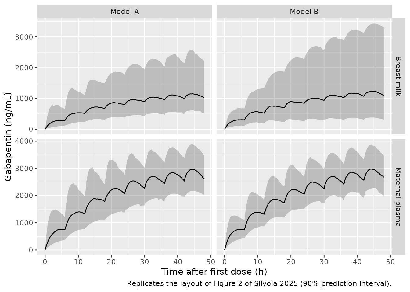
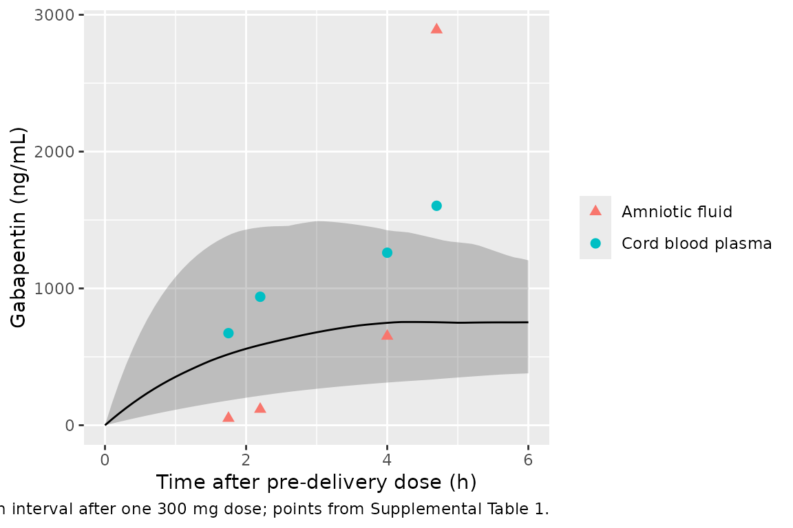
Figure 3 and Supplemental Table 1: cord blood against maternal plasma
Figure 3 compares predicted maternal plasma concentrations with the cord blood and amniotic fluid concentrations measured after the single pre-delivery dose (Supplemental Table 1). Cord blood at delivery should sit at or below the maternal plasma prediction band for the corresponding time after dose.
cord <- tibble::tribble(
  ~subject, ~time, ~amniotic, ~cord,
  104, 4.7, 2890, 1604,
  107, 2.2, 117, 939,
  110, 1.75, 51, 673,
  112, 4, 651, 1261
)

sim_a |>
  filter(time <= 6) |>
  group_by(time) |>
  summarise(
    Q05 = quantile(Cc * 1000, 0.05),
    Q50 = median(Cc * 1000),
    Q95 = quantile(Cc * 1000, 0.95),
    .groups = "drop"
  ) |>
  ggplot(aes(time, Q50)) +
  geom_ribbon(aes(ymin = Q05, ymax = Q95), alpha = 0.25) +
  geom_line() +
  geom_point(data = cord, aes(time, cord, colour = "Cord blood plasma"), size = 2) +
  geom_point(data = cord, aes(time, amniotic, colour = "Amniotic fluid"), size = 2, shape = 17) +
  labs(
    x = "Time after pre-delivery dose (h)", y = "Gabapentin (ng/mL)", colour = NULL,
    caption = "Model A maternal plasma 90% prediction interval after one 300 mg dose; points from Supplemental Table 1."
  )
PKNCA validation
Table 4 of the paper reports, for each model, the median and 95%
prediction interval of the average maternal plasma and breast-milk
concentrations on day 1 (0-24 h) and day 2 (24-48 h). The average
concentration over an interval is the PKNCA parameter cav
(AUC over the interval divided by its length), so PKNCA is run once per
matrix with one interval per day.
doses <- bind_rows(
  ev_a |> filter(evid == 1) |> mutate(model = "Model A"),
  ev_b |> filter(evid == 1) |> mutate(model = "Model B")
) |>
  select(id, time, amt, model)

intervals <- data.frame(start = c(0, 24), end = c(24, 48), cav = TRUE, auclast = TRUE)

run_nca <- function(conc_col) {
  conc <- sim |>
    filter(!is.na(.data[[conc_col]])) |>
    select(id, time, model, conc = all_of(conc_col))
  conc_obj <- PKNCA::PKNCAconc(conc, conc ~ time | model + id)
  dose_obj <- PKNCA::PKNCAdose(doses, amt ~ time | model + id)
  res <- PKNCA::pk.nca(PKNCA::PKNCAdata(conc_obj, dose_obj, intervals = intervals))
  as.data.frame(res) |>
    mutate(day = ifelse(start == 0, "Day 1", "Day 2"))
}

nca_plasma <- run_nca("Cc") |> mutate(matrix = "Maternal plasma")
nca_milk <- run_nca("Cmilk") |> mutate(matrix = "Breast milk")
nca <- bind_rows(nca_plasma, nca_milk)
Comparison against Table 4
# Table 4 medians, converted from ng/mL to mg/L (the model's units).
published <- tibble::tribble(
  ~model, ~matrix, ~day, ~cav,
  "Model A", "Maternal plasma", "Day 1", 1480,
  "Model A", "Maternal plasma", "Day 2", 2650,
  "Model A", "Breast milk", "Day 1", 582,
  "Model A", "Breast milk", "Day 2", 1060,
  "Model B", "Maternal plasma", "Day 1", 1450,
  "Model B", "Maternal plasma", "Day 2", 2640,
  "Model B", "Breast milk", "Day 1", 580,
  "Model B", "Breast milk", "Day 2", 1070
) |>
  mutate(cav = cav / 1000)

sim_cav <- nca |>
  filter(PPTESTCD == "cav") |>
  select(model, matrix, day, PPTESTCD, PPORRES)

cmp <- nlmixr2lib::ncaComparisonTable(
  simulated = sim_cav,
  reference = published,
  by = c("model", "matrix", "day"),
  units = c(cav = "mg/L"),
  tolerance_pct = 20
)
knitr::kable(cmp, caption = "Median average concentration per day: simulated (200 women) vs Table 4 (10,000 women).")| NCA parameter | model | matrix | day | Reference | Simulated | % diff |
|---|---|---|---|---|---|---|
| Cavg (mg/L) | Model A | Maternal plasma | Day 1 | 1.48 | 1.46 | -1.6% |
| Cavg (mg/L) | Model A | Maternal plasma | Day 2 | 2.65 | 2.64 | -0.4% |
| Cavg (mg/L) | Model A | Breast milk | Day 1 | 0.582 | 0.556 | -4.5% |
| Cavg (mg/L) | Model A | Breast milk | Day 2 | 1.06 | 1.03 | -3.1% |
| Cavg (mg/L) | Model B | Maternal plasma | Day 1 | 1.45 | 1.44 | -0.4% |
| Cavg (mg/L) | Model B | Maternal plasma | Day 2 | 2.64 | 2.64 | +0.2% |
| Cavg (mg/L) | Model B | Breast milk | Day 1 | 0.58 | 0.578 | -0.3% |
| Cavg (mg/L) | Model B | Breast milk | Day 2 | 1.07 | 1.08 | +1.3% |
pct <- sim_cav |>
  group_by(model, matrix, day) |>
  summarise(sim = median(PPORRES), .groups = "drop") |>
  inner_join(published, by = c("model", "matrix", "day")) |>
  mutate(pct_diff = 100 * (sim / cav - 1))
stopifnot(
  nrow(pct) == 8,
  # A mis-transcribed CL/F, V/F, MPR or milk rate constant, or a ng/mL vs mg/L
  # slip, moves these medians by tens of percent or more. With 200 women the
  # Monte Carlo error of a median is a few percent (milk BSV is largest).
  all(abs(pct$pct_diff) < 10)
)
The 95% prediction intervals from the same simulation, set beside Table 4:
nca |>
  filter(PPTESTCD == "cav") |>
  group_by(model, matrix, day) |>
  summarise(
    sim = sprintf(
      "%.0f (%.0f-%.0f)", 1000 * median(PPORRES),
      1000 * quantile(PPORRES, 0.025), 1000 * quantile(PPORRES, 0.975)
    ),
    .groups = "drop"
  ) |>
  left_join(
    tibble::tribble(
      ~model, ~matrix, ~day, ~table4,
      "Model A", "Maternal plasma", "Day 1", "1480 (695-2460)",
      "Model A", "Maternal plasma", "Day 2", "2650 (1770-3660)",
      "Model A", "Breast milk", "Day 1", "582 (206-1510)",
      "Model A", "Breast milk", "Day 2", "1060 (446-2430)",
      "Model B", "Maternal plasma", "Day 1", "1450 (830-2250)",
      "Model B", "Maternal plasma", "Day 2", "2640 (1880-3600)",
      "Model B", "Breast milk", "Day 1", "580 (186-1810)",
      "Model B", "Breast milk", "Day 2", "1070 (314-3610)"
    ),
    by = c("model", "matrix", "day")
  ) |>
  rename(
    "Model" = model, "Matrix" = matrix, "Day" = day,
    "Simulated median (95% PI), ng/mL" = sim,
    "Table 4 median (95% PI), ng/mL" = table4
  ) |>
knitr::kable()| Model | Matrix | Day | Simulated median (95% PI), ng/mL | Table 4 median (95% PI), ng/mL |
|---|---|---|---|---|
| Model A | Breast milk | Day 1 | 556 (208-1585) | 582 (206-1510) |
| Model A | Breast milk | Day 2 | 1027 (443-2406) | 1060 (446-2430) |
| Model A | Maternal plasma | Day 1 | 1456 (741-2385) | 1480 (695-2460) |
| Model A | Maternal plasma | Day 2 | 2638 (1771-3628) | 2650 (1770-3660) |
| Model B | Breast milk | Day 1 | 578 (166-1884) | 580 (186-1810) |
| Model B | Breast milk | Day 2 | 1083 (288-4044) | 1070 (314-3610) |
| Model B | Maternal plasma | Day 1 | 1444 (819-2148) | 1450 (830-2250) |
| Model B | Maternal plasma | Day 2 | 2645 (1844-3588) | 2640 (1880-3600) |
Maternal AUC over 48 h
The Results report a mean (SD) maternal plasma AUC0-48h of 103.7 (32.2) mg*h/L, median 98.2, from the individual Model A estimates of the 20 women.
auc48 <- nca_plasma |>
  filter(PPTESTCD == "auclast", model == "Model A") |>
  group_by(id) |>
  summarise(auc048 = sum(PPORRES), .groups = "drop")
summary(auc48$auc048)
#>    Min. 1st Qu.  Median    Mean 3rd Qu.    Max.
#>   53.57   85.51   99.32  100.22  116.32  153.00
stopifnot(abs(median(auc48$auc048) / 98.2 - 1) < 0.15)
Infant daily dose and relative infant dose
The paper computes the infant daily dose as the day-average milk concentration times the daily milk intake (4 mL/kg on day 1, 13 mL/kg on day 2) and the relative infant dose as the infant daily dose over a maternal daily dose of 12.3 mg/kg/day (1200 mg/day at 97.7 kg).
intake <- c("Day 1" = 4, "Day 2" = 13) # mL/kg/day
mdd <- 12.3 # mg/kg/day

infant <- nca_milk |>
  filter(PPTESTCD == "cav") |>
  mutate(
    idd = PPORRES * intake[day] / 1000, # mg/L x mL/kg / 1000 = mg/kg/day
    rid = 100 * idd / mdd
  ) |>
  group_by(model, day) |>
  summarise(idd = median(idd), rid = median(rid), .groups = "drop") |>
  left_join(
    tibble::tribble(
      ~model, ~day, ~idd_pub, ~rid_pub,
      "Model A", "Day 1", 0.00233, 0.0189,
      "Model A", "Day 2", 0.0137, 0.112,
      "Model B", "Day 1", 0.00232, 0.0189,
      "Model B", "Day 2", 0.0139, 0.113
    ),
    by = c("model", "day")
  )

infant |>
  rename(
    "Model" = model, "Day" = day,
    "IDD simulated (mg/kg/day)" = idd, "IDD Table 4" = idd_pub,
    "RID simulated (%)" = rid, "RID Table 4" = rid_pub
  ) |>
knitr::kable(digits = 5)| Model | Day | IDD simulated (mg/kg/day) | RID simulated (%) | IDD Table 4 | RID Table 4 |
|---|---|---|---|---|---|
| Model A | Day 1 | 0.00222 | 0.01807 | 0.00233 | 0.0189 |
| Model A | Day 2 | 0.01335 | 0.10854 | 0.01370 | 0.1120 |
| Model B | Day 1 | 0.00231 | 0.01881 | 0.00232 | 0.0189 |
| Model B | Day 2 | 0.01409 | 0.11451 | 0.01390 | 0.1130 |
The paper’s Table 4 arithmetic is itself reproducible from its milk concentrations: 582 ng/mL x 4 mL/kg = 0.00233 mg/kg/day, and 0.00233 / 12.3 = 0.0189%, which confirms that the reported breast-milk concentration is the day-average concentration.
Assumptions and deviations
-
The absorption rate constant is a multiple of kel.
Both control streams set
TVKA = THETA(1)*KEwithTHETA(1)bounded below by 1, which is how the authors constrained ka to exceed ke and excluded the flip-flop solution their unconstrained fit found (Results 3.1). Tables 2 and 3 print only the derived product (0.43 and 0.51/h), so the ratio is back-solved aska / (CL/F / V2/F): 7.828 for Model A and 9.904 for Model B. The packaged models keep this form, through the canonicallkaratio/karatiothat the maintainers ratified for it, with the lower bound of 1 written asc(0, log(...))on the log scale. Because between-subject variability sits on CL/F and V/F, each woman’s ka follows her own kel; a freelkawould give the same typical profile but a narrower absorption-phase spread. -
No BSV on ka. Data S1 carries
$OMEGA 0 FIXfor ka; the paper retained BSV on CL/F and V/F “but not ka”. The packaged models have noetalka. -
Data S2 is truncated. The published Model B control
stream stops inside
$ERROR, so its$THETA,$OMEGAand$SIGMAblocks are missing. Every final estimate comes from Table 3, and the proportional error model is taken from the*prop*tag in its$PROBLEMline and the complete Model A stream. -
Figure 1 writes Model A’s milk equation on amounts
(
A_BreastMilk = MPR x A_c). MPR is a concentration ratio (Figure 1 caption, Methods 2.6) and the Data S1$ERRORblock computesIPRED = (A(2)/S2)*MPR, a concentration, so the packaged model usesCmilk <- cmpr * Cc. -
Units. The source reports ng/mL; the models use mg
dose and L volumes, so concentrations are in mg/L (1 mg/L = 1000 ng/mL).
The control streams’
S2 = V2/1000scaling is the same conversion. -
Dosing in the Table 4 simulation. The paper states
only “300 mg of gabapentin every 6 h” for 48 h. The simulation here
doses at 0, 6, …, 42 h with time zero at the first dose, and day 1 and
day 2 are 0-24 h and 24-48
- Figure 3 caption says “every 8 h”, whereas the protocol (Methods 2.1), the Methods 2.7 simulation and the 1200 mg/day maternal dose all say every 6 h; the caption is taken to be a typographical error.
- Median maternal weight. Table 1 gives 107.5 kg for the 21 enrolled women, while the Table 4 footnote uses 97.7 kg to derive the maternal daily dose of 12.3 mg/kg/day. Neither enters the model; the 12.3 mg/kg/day used here reproduces the paper’s relative infant doses.
-
Covariates. Weight, BMI, eGFR and time after
delivery were explored graphically but not retained because they
destabilised the model; they are recorded under
covariatesDataExcludedin both model files. - Cohort size. 200 simulated women per model instead of the paper’s 10,000; the medians agree within the Monte Carlo error of that sample size.