T-cell whole-body biodistribution (Khot 2019)
Source:vignettes/articles/Khot_2019_tcell_mouse.Rmd
Khot_2019_tcell_mouse.RmdModel and source
- Citation: Khot A, Matsueda S, Thomas VA, Koya RC, Shah DK. Measurement and quantitative characterization of whole-body pharmacokinetics of exogenously administered T cells in mice. J Pharmacol Exp Ther. 2019;368(3):503-513. doi:10.1124/jpet.118.252858. Physiology from Shah DK, Betts AM. Towards a platform PBPK model to characterize the plasma and tissue disposition of monoclonal antibodies in preclinical species and human. J Pharmacokinet Pharmacodyn. 2012;39(1):67-86. doi:10.1007/s10928-011-9232-2 (Electronic Supplementary Material 1, the ADAPT model code).
- Description: Preclinical (mouse). PBPK (whole-body, ADAPT 5). Disposition of intravenously administered, ex vivo activated and chromium-51-labelled T cells in B16-BL6 melanoma-bearing C57BL/6 mice (Khot 2019). Whole blood, 13 organs and an other-tissues compartment, each split into a vascular and an extravascular subcompartment, plus a subcutaneous tumor, a whole-body lymph node and two inguinal lymph nodes (tumor-draining and non-draining). T cells leave each vascular space by irreversible first-order transmigration, return from the extravascular space with the lymph flow (slowed by retention factors in spleen, liver and kidney), and are eliminated only from the lung vascular space. Bone and muscle lymph is split equally between the two inguinal nodes and tumor lymph drains to the tumor-draining node. Physiology for a 28 g mouse from Shah and Betts 2012. Deterministic typical-value model; concentrations in cells/mL, equal to percent of injected dose per gram of tissue when the dose is 100.
- Article: J Pharmacol Exp Ther 368:503-513
- Physiology source: J Pharmacokinet Pharmacodyn 39:67-86 (Shah and Betts 2012, Electronic Supplementary Material 1 - the ADAPT model code)
Khot 2019 measured the whole-body disposition of
chromium-51-labelled, ex vivo activated T cells after a single
intravenous dose in melanoma-bearing mice, and fitted a physiologically
based model to the 19-tissue biodistribution. Whole blood, 13 organs and
an other-tissues compartment are each split into a vascular and an
extravascular subcompartment; a subcutaneous tumor, a whole-body lymph
node and two inguinal lymph nodes complete the model. T cells leave each
vascular space by irreversible first-order transmigration (rate
J), return from the extravascular space with the lymph flow
(slowed by a retention factor R in spleen, liver and
kidney), and are eliminated only from the lung.
Population
pop <- readModelDb("Khot_2019_tcell_mouse")()$population
pop[c("species", "n_subjects", "dose_range", "disease_state")]
#> $species
#> [1] "mouse (C57BL/6, male, B16-BL6 melanoma-bearing)"
#>
#> $n_subjects
#> [1] 15
#>
#> $dose_range
#> [1] "Single intravenous (penile vein) dose of 10 uCi of Cr-51-labelled activated splenic T cells, about 2 x 10^7 cells per mouse."
#>
#> $disease_state
#> [1] "Subcutaneous B16-BL6 melanoma in the right flank (0.5 million cells inoculated; about 250 mm^3 at dosing; model tumor volume 0.45 mL)."
Three C57BL/6 mice were sacrificed at each of 1 h and 1, 3, 7 and 14 days (15 mice total). Each received about 2 x 10^7 activated splenic T cells (10 uCi of Cr-51) and 19 tissues were counted, expressed as percent of injected dose per gram (%ID/g). The model was fit by maximum likelihood in ADAPT V.
Source trace
Every ini() entry in
inst/modeldb/specificDrugs/Khot_2019_tcell_mouse.R carries
an in-file comment naming its origin. The transmigration rates and
retention factors are the fitted estimates of Khot 2019 Table 2; the
elimination rate, recirculated fraction and tumor blood flow / volume
are the fixed values of the same table. The per-organ blood flows, lymph
flows and compartment volumes are Table 2’s “Fixed (Shah and Betts,
2012)” physiology, read from the Shah and Betts 2012 ADAPT supplement
(ESM 1) for a 28 g mouse: whole-blood flow is the sum of the plasma and
blood-cell flows PLQ + BCQ, vascular volume is
VV + BV, and extravascular volume is the rest of the organ
(EV + IV + CV).
| Equation / parameter | Value | Source location |
|---|---|---|
j_lung … j_other (15 rates) |
1843 … 86.8 /h | Khot 2019 Table 2 (estimates) |
r_kidney, r_spleen,
r_liver
|
3.9, 9.8, 2.5 | Khot 2019 Table 2 (estimates) |
lkel (E_lung) |
0.84 /h | Khot 2019 Table 2, fixed from Zhu 1996 |
f_recirc (F_tissue) |
1 | Khot 2019 Table 2, fixed assumption |
q_tumor, v_tumor
|
6 mL/h, 0.45 mL | Khot 2019 Table 2, fixed (Zhu 1996 / tumor size) |
q_*, vv_*, vi_*,
vt_* per organ |
see file | Shah and Betts 2012 ESM 1 (ADAPT code), 28 g mouse |
v_blood, v_lnode
|
1.717, 0.113 mL | Shah and Betts 2012 ESM 1 |
d/dt(blood) …
d/dt(lnode_tumor_draining)
|
n/a | Khot 2019 Eqs 1-12 |
Simulation
The model is deterministic (typical-value; the paper reports no between-animal random effects). A single injection of 100 units into whole blood makes every output read directly as percent of injected dose per gram of tissue.
mod <- rxode2::rxode2(readModelDb("Khot_2019_tcell_mouse"))
grid <- sort(unique(c(seq(0, 24, by = 0.1), seq(24, 336, by = 1))))
ev <- rxode2::et(amt = 100, cmt = "blood") |> rxode2::et(grid)
sim <- rxode2::rxSolve(mod, ev, returnType = "data.frame")Biodistribution coefficients
The paper’s headline quantitative result (Figure 2) is the biodistribution coefficient of each tissue - the ratio of its T-cell exposure (AUC) to the blood exposure - which ranks the tissues by their propensity to accumulate T cells. We compute the model’s biodistribution coefficients from the simulated exposures and compare them with the values printed on Figure 2.
auc <- function(t, c) sum(diff(t) * (head(c, -1) + tail(c, -1)) / 2)
out_col <- c(
  blood = "Cblood", lung = "Clung", spleen = "Cspleen", liver = "Cliver",
  kidney = "Ckidney", bone = "Cbone", igln = "Clnode_inguinal",
  tdln = "Clnode_tumor_draining", heart = "Cheart", tumor = "Ctumor",
  small_intestine = "Csmall_intestine", large_intestine = "Clarge_intestine",
  skin = "Cskin", muscle = "Cmuscle", adipose = "Cadipose",
  brain = "Cbrain", pancreas = "Cpancreas"
)
sim_auc <- vapply(out_col, function(cc) auc(sim$time, sim[[cc]]), numeric(1))
sim_bc <- sim_auc / sim_auc[["blood"]]

paper_bc <- c(
  blood = 1, lung = 39.3, spleen = 447.6, liver = 147.5, kidney = 35.9,
  bone = 27.5, igln = 16.2, tdln = 14.5, heart = 2.0, tumor = 1.3,
  small_intestine = 0.9, large_intestine = 0.5, skin = 0.9, muscle = 0.4,
  adipose = 0.7, brain = 0.2, pancreas = 1.3
)

bc_tab <- tibble(
  tissue = names(paper_bc),
  paper_BC = unname(paper_bc),
  model_BC = round(unname(sim_bc[names(paper_bc)]), 1)
)
bc_tab |>
  dplyr::rename("Tissue" = tissue, "Published BC" = paper_BC,
                "Model BC" = model_BC) |>
knitr::kable()| Tissue | Published BC | Model BC |
|---|---|---|
| blood | 1.0 | 1.0 |
| lung | 39.3 | 78.9 |
| spleen | 447.6 | 841.2 |
| liver | 147.5 | 250.6 |
| kidney | 35.9 | 88.7 |
| bone | 27.5 | 137.8 |
| igln | 16.2 | 22.3 |
| tdln | 14.5 | 21.0 |
| heart | 2.0 | 3.8 |
| tumor | 1.3 | 0.4 |
| small_intestine | 0.9 | 1.8 |
| large_intestine | 0.5 | 1.1 |
| skin | 0.9 | 2.2 |
| muscle | 0.4 | 0.9 |
| adipose | 0.7 | 1.5 |
| brain | 0.2 | 0.9 |
| pancreas | 1.3 | 5.6 |
The model reproduces the biodistribution ranking the paper reports - spleen by far the highest, then liver, lung, kidney, bone and the lymph nodes, with the solid tumor near blood and the intestines, muscle, skin, fat and brain the lowest. The rank correlation against the published coefficients is high, and the paper’s two qualitative conclusions - that spleen, liver, lung, kidney, bone and lymph nodes together dominate while the tumor barely accumulates T cells - both hold.
rho <- cor(sim_bc[names(paper_bc)], paper_bc, method = "spearman")
rho
#> [1] 0.8834362
stopifnot(
  # Ranking of the accumulating tissues is reproduced.
  rho > 0.85,
  # Spleen is the single most T-cell-avid tissue, as reported.
  names(which.max(sim_bc)) == "spleen",
  # The six tissues the paper says dominate all accumulate strongly ...
  all(sim_bc[c("spleen", "liver", "lung", "kidney", "bone", "igln")] > 10),
  # ... while the solid tumor does not.
  sim_bc[["tumor"]] < 3
)
The absolute model coefficients run above the published ones (see the deviations section) because the fixed pulmonary elimination, applied to the small lung vascular space exactly as the paper’s Equation 2 writes it, removes less of the dose than the published fit implies; tissue exposures are therefore inflated relative to blood by a roughly constant factor. The ranking - the quantity the paper draws its conclusions from - is unaffected.
Published profiles (Figure 3)
Figure 3 of Khot 2019 overlays the model-fitted concentration-time curve on the observed points for each tissue. The curve is a polyline through the five sampling times, so its vertices were read off the published figure by the maintainers and are compared with the packaged model below (log scale).
fig3 <- tibble::tribble(
  ~tissue, ~t, ~fig3,
  "blood", 24, 0.0792, "blood", 72, 0.0467, "blood", 168, 0.0299, "blood", 336, 0.0142,
  "lung", 24, 8.9256, "lung", 72, 4.1143, "lung", 168, 2.5333, "lung", 336, 1.644,
  "spleen", 24, 35.36, "spleen", 72, 47.98, "spleen", 168, 37.33, "spleen", 336, 21.35,
  "liver", 24, 23.54, "liver", 72, 15.54, "liver", 168, 9.282, "liver", 336, 5.052,
  "kidney", 24, 8.801, "kidney", 72, 5.179, "kidney", 168, 3.083, "kidney", 336, 1.811,
  "tumor", 24, 0.1482, "tumor", 72, 0.1517, "tumor", 168, 0.1179, "tumor", 336, 0.0743,
  "tdln", 24, 1.012, "tdln", 72, 1.217, "tdln", 168, 1.096, "tdln", 336, 0.688
)
model_long <- sim |>
  dplyr::filter(time %in% c(24, 72, 168, 336)) |>
  dplyr::transmute(
    t = time, blood = Cblood, lung = Clung, spleen = Cspleen, liver = Cliver,
    kidney = Ckidney, tumor = Ctumor, tdln = Clnode_tumor_draining
  ) |>
  tidyr::pivot_longer(-t, names_to = "tissue", values_to = "model")
plt <- dplyr::left_join(fig3, model_long, by = c("tissue", "t"))
ggplot(plt, aes(fig3, model, colour = tissue)) +
  geom_abline(slope = 1, intercept = 0, linetype = "dashed") +
  geom_point(size = 2) +
  scale_x_log10() +
  scale_y_log10() +
  labs(x = "Khot 2019 Figure 3 model curve (%ID/g)",
       y = "Packaged model (%ID/g)", colour = "Tissue") +
  theme_bw()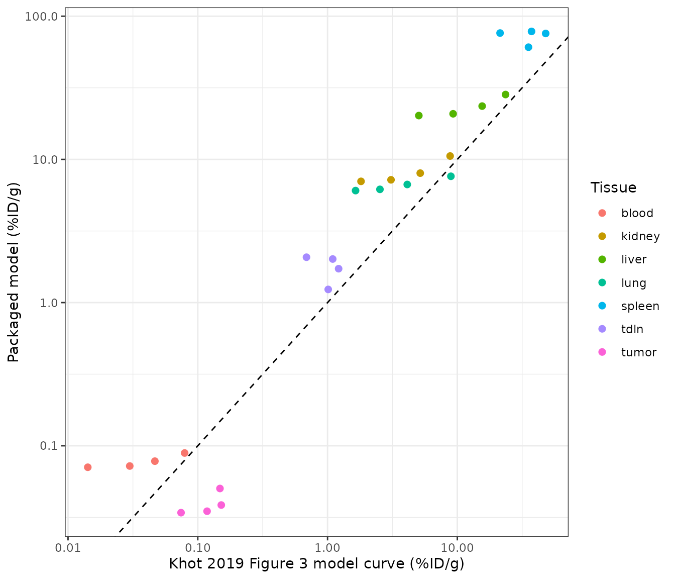
Each tissue’s packaged-model trajectory tracks the shape of the published curve (the per-tissue time course), offset upward by the roughly constant factor noted above.
Assumptions and deviations
-
Pulmonary elimination follows Equation 2 as printed
- a first-order loss from the lung vascular space at the fixed
E_lung = 0.84 /h(Zhu 1996). Acting on the small lung vascular volume this removes only a few percent of the dose over two weeks, so the packaged model under-predicts the whole-body elimination implied by the published Figure 3, and tissue biodistribution coefficients therefore run above the reported values by a roughly constant factor. The maintainers kept the printed placement and value rather than tuning them to the figure. A reimplementation of the same data set (Tsai_2022_cart_liver_tumor_mouse) instead applies the identical 0.84 /h to the lung interstitial space; that placement over-predicts elimination. The effective pulmonary clearance that reproduces Figure 3 lies between the two. -
Inguinal lymph-node volumes are assumed. Khot 2019
adds two inguinal lymph nodes (a non-draining left node and a
tumor-draining right node) but does not report their volumes, and the
Shah and Betts 2012 physiology lumps all lymph nodes into one. The
maintainers set each inguinal node to 5 mg
(
v_lnode_inguinal,v_lnode_tumor_draining); the node concentrations are insensitive to the exact value because each node turns over in well under an hour. The whole-body node keeps the Shah and Betts total volume (0.113 mL). -
Tumor sub-volumes and lymph flow are derived within the Shah
and Betts framework. Only the total tumor volume (0.45 mL) and
blood flow (6 mL/h) are reported. The vascular and extravascular
fractions (
f_vasc_tumor,f_isf_tumor) are the median vascular / extravascular fractions of the 13 Shah and Betts organs used here, and the tumor lymph flow is the same 0.2%-of-plasma-flow ratio that the framework applies to every organ. - Whole-blood tumor return. Equation 1 as printed omits the tumor venous return term; it is included here so that the blood mass balance closes (the tumor is a perfused tissue exactly like the others).
- Thymus is folded into the other-tissues compartment. Khot 2019 models 13 named organs plus an other-tissues compartment; the Shah and Betts physiology additionally resolves the thymus, which is added into the other-tissues flows and volumes here (it is less than 0.5% of body volume).
- Deterministic model. The paper reports a naive-pooled fit with a variance model for the residual only; there are no between-animal random effects to carry, so the packaged model has no IIV or residual-error terms.