Doxorubicin (Perez-Blanco 2016)
Source:vignettes/articles/PerezBlanco_2016_doxorubicin.Rmd
PerezBlanco_2016_doxorubicin.RmdModel and source
- Citation: Perez-Blanco JS, Santos-Buelga D, Fernandez de Gatta MM, Hernandez-Rivas JM, Martin A, Garcia MJ. Population pharmacokinetics of doxorubicin and doxorubicinol in patients diagnosed with non-Hodgkin’s lymphoma. Br J Clin Pharmacol. 2016;82(6):1517-1527. doi:10.1111/bcp.13070
- Article: https://doi.org/10.1111/bcp.13070
Population
Perez-Blanco 2016 enrolled 45 adult patients with non-Hodgkin’s
lymphoma (diffuse large B-cell lymphoma n = 36, Burkitt-like lymphoma n
= 2, follicular lymphoma n = 2, other n = 5) treated with the R-CHOP
regimen at six Spanish hospitals between June 2009 and June 2015.
Patients received doxorubicin as a 0.5-h IV infusion (range 0.2-1.3 h)
at a protocol dose of 50 mg/m^2 every 21 days for six cycles, supported
with G-CSF prophylaxis where indicated. Baseline demographics from Table
1: age 26-84 years (mean 66, SD 15), weight 43-110 kg (mean 71), height
1.43-1.92 m (mean 1.64), body surface area 1.3-2.3 m^2 (mean 1.8), and a
nearly balanced sex split (22 female / 23 male). All patients had normal
hepatic, renal, and cardiac function. Sparse PK sampling was performed
at 0, 30, 90, and 180 min after the end of each studied infusion,
yielding 125 doxorubicin and 120 doxorubicinol plasma concentrations for
the population fit (one outlier subject with |CWRES| > 4 removed, n =
44 in the final fit). The UHPLC-fluorescence assay’s lower limit of
quantification was 8 ng/mL for doxorubicin and 3 ng/mL for
doxorubicinol. The same information is available programmatically via
rxode2::rxode(readModelDb("PerezBlanco_2016_doxorubicin"))$population.
Source trace
Final parameter estimates come from Perez-Blanco 2016 Table 2 column “Final model (n = 44)”. Five volumes are FIXED: the DOX volumes V1, V2, V3 to the Kontny 2013 (doi:10.1007/s00280-013-2261-3) adult-reference values; the DOXol volumes V4 and V5 to the values obtained from the authors’ sensitivity analysis. Three IIVs (Q2, Q3, CLm) are also FIXED at their model-building values to avoid over-parameterisation.
| Equation / parameter | Value | Source location |
|---|---|---|
lcl (CL doxorubicin total) |
62.4 L/h | Table 2 row 1, RSE 11.5% |
lvc (V1 doxorubicin central) |
17.7 L FIXED | Table 2 row 2 FIX, from Kontny 2013 |
lq (Q2 doxorubicin) |
50.7 L/h | Table 2 row 3, RSE 18.4% |
lvp (V2 doxorubicin peripheral1) |
1830 L FIXED | Table 2 row 4 FIX, from Kontny 2013 |
lq2 (Q3 doxorubicin) |
28.4 L/h | Table 2 row 5, RSE 13.5% |
lvp2 (V3 doxorubicin peripheral2) |
71 L FIXED | Table 2 row 6 FIX, from Kontny 2013 |
lfm (Fm fraction metabolised) |
0.22 | Table 2 row 9, RSE 14.7% |
lcl_doxol (CLm doxorubicinol) |
26.8 L/h | Table 2 row 8, RSE 42.9% |
lvc_doxol (V4 doxorubicinol central) |
79.8 L FIXED | Table 2 row 7 FIX, sensitivity analysis |
lvp_doxol (V5 doxorubicinol peripheral1) |
653 L FIXED | Table 2 row 10 FIX, sensitivity analysis |
lq_doxol (Q5 doxorubicinol) |
424 L/h | Table 2 row 11, RSE 18.0% |
| IIV(CL) | 22.9% CV -> omega^2 = 0.0511 | Table 2 row 12, RSE 32.7%, shrinkage 40% |
| IIV(Q2) FIXED | 64.1% CV -> omega^2 = 0.3442 | Table 2 row 13 FIX |
| IIV(Q3) FIXED | 28.2% CV -> omega^2 = 0.0765 | Table 2 row 14 FIX |
| IIV(CLm) FIXED | 47.2% CV -> omega^2 = 0.2011 | Table 2 row 15 FIX |
| IIV(Fm) | 41.7% CV -> omega^2 = 0.1603 | Table 2 row 16, RSE 19.6%, shrinkage 22% |
| IIV(Q5) | 58.9% CV -> omega^2 = 0.2978 | Table 2 row 17, RSE 39.4%, shrinkage 35% |
| Proportional residual SD (DOX) | 0.371 (= 37.1%) | Table 2 row 18, RSE 8.3%, shrinkage 15% |
| Proportional residual SD (DOXol) | 0.321 (= 32.1%) | Table 2 row 19, RSE 10.4%, shrinkage 21% |
d/dt(central) 3-cmt IV, parent loss
-cl/vc * central
|
– | Methods ‘popPK analysis’; Figure 2 schematic |
d/dt(central_doxol) input
fm * cl / vc * central
|
– | AUCm = Dose * Fm / CLm (Methods ‘Drug exposure and haematological toxicity’) |
The Value column shows the typical-value parameter
estimate; the in-file comments next to each ini() entry pin
every value to the same locations.
Virtual cohort
Original patient-level concentrations are not publicly available. The
cohort below is reconstructed to match Table 1 demographics: n = 45,
mean BSA 1.8 m^2, mean weight 71 kg, mean age 66 years, balanced sex
ratio. Because the final model retained no covariates, the only
quantities that flow into rxSolve are the dose
(proportional to BSA) and the infusion duration (0.5 h); the demographic
columns are carried for completeness and to feed the figures.
set.seed(20160929)  # Perez-Blanco 2016 BJCP published-online date

n_sub <- 45L

# Approximate the Table 1 distributions with a normal draw clipped to
# the published ranges. The exact patient-level values are not
# available; this is the best-feasible virtual reconstruction.
clip <- function(x, lo, hi) pmin(pmax(x, lo), hi)

cohort <- tibble::tibble(
  id  = seq_len(n_sub),
  AGE = clip(rnorm(n_sub, mean = 66, sd = 15), 26,   84),
  WT  = clip(rnorm(n_sub, mean = 71, sd = 12), 43,  110),
  BSA = clip(rnorm(n_sub, mean = 1.8, sd = 0.2), 1.3, 2.3),
  SEXF = c(rep(1L, 22), rep(0L, 23))[sample.int(n_sub)],
  DOSE_MG_M2 = 50,            # protocol dose
  INF_DUR_H  = 0.5            # protocol infusion duration
) |>
  dplyr::mutate(
    DOSE_MG = DOSE_MG_M2 * BSA,
    treatment = "50 mg/m^2 IV over 0.5 h"
  )

# Observation grid: dense early to capture distribution and the
# infusion ramp, then logarithmic out to 168 h for the terminal phase.
obs_times <- c(
  seq(0.05, 0.5,  length.out = 12),
  seq(0.6,  6.0,  length.out = 25),
  seq(8,    24,   length.out = 12),
  seq(36,   168,  length.out = 12)
)

events <- cohort |>
  dplyr::rowwise() |>
  dplyr::do({
    s <- .
    dplyr::bind_rows(
      tibble::tibble(id = s$id, time = 0,         amt = s$DOSE_MG,
                     dur  = s$INF_DUR_H, evid = 1L, cmt = "central"),
      tibble::tibble(id = s$id, time = obs_times, amt = NA_real_,
                     dur  = NA_real_,    evid = 0L, cmt = "Cc")
    ) |>
      dplyr::mutate(
        AGE = s$AGE, WT = s$WT, BSA = s$BSA, SEXF = s$SEXF,
        DOSE_MG_M2 = s$DOSE_MG_M2,
        treatment  = s$treatment
      )
  }) |>
  dplyr::ungroup() |>
  as.data.frame()

stopifnot(!anyDuplicated(unique(events[, c("id", "time", "evid")])))
Simulation
The figures below use typical-value predictions (zero between-subject variability) to reproduce the structural-model behaviour, and a separate stochastic VPC with the full IIV / residual structure for prediction spread. The original Figures 2-3 in the paper are pcVPCs built from patient-level fits; we approximate the typical-value overlays here.
mod        <- rxode2::rxode(readModelDb("PerezBlanco_2016_doxorubicin"))
#> ℹ parameter labels from comments will be replaced by 'label()'
mod_typ    <- rxode2::zeroRe(mod)

sim_typical <- rxode2::rxSolve(
  mod_typ,
  events = events,
  keep   = c("AGE", "WT", "BSA", "SEXF", "DOSE_MG_M2", "treatment")
) |>
  as.data.frame() |>
  dplyr::filter(time > 0)
#> ℹ omega/sigma items treated as zero: 'etalcl', 'etalq', 'etalq2', 'etalfm', 'etalcl_doxol', 'etalq_doxol'
#> Warning: multi-subject simulation without without 'omega'
# Stochastic VPC with the full IIV structure. Keep nSub small so the
# vignette renders under the 5-minute pkgdown gate.
ev_one <- events |>
  dplyr::filter(id == 1L) |>
  dplyr::select(time, amt, dur, evid, cmt) |>
  rxode2::et()

sim_vpc <- rxode2::rxSolve(mod, events = ev_one, nSub = 200) |>
  as.data.frame()
Replicate published figures
Figure 2 – Doxorubicin and doxorubicinol typical-value profiles
sim_long <- sim_typical |>
  tidyr::pivot_longer(c(Cc, Cc_doxol),
                      names_to = "analyte", values_to = "conc") |>
  dplyr::mutate(
    analyte = dplyr::recode(analyte,
                            Cc       = "Doxorubicin",
                            Cc_doxol = "Doxorubicinol"),
    conc_ngml = conc * 1000     # mg/L -> ng/mL for visual alignment with paper Figs 2-3
  )

ggplot(sim_long, aes(time, conc_ngml, group = id)) +
  geom_line(alpha = 0.5, colour = "steelblue") +
  facet_wrap(~analyte, scales = "free_y") +
  scale_y_log10() +
  scale_x_continuous(limits = c(0, 24)) +
  labs(x = "Time after dose end (h)",
       y = "Plasma concentration (ng/mL)",
       title = "Typical-value profiles per virtual subject",
       caption = paste("Replicates the shape of Figure 2 (pcVPC) in Perez-Blanco 2016 for the typical 50 mg/m^2 IV dose over 0.5 h.",
                       "Subjects differ only in BSA-scaled dose; structural model is identical because no covariate effects were retained.",
                       sep = " "))
#> Warning: Removed 1080 rows containing missing values or values outside the scale range
#> (`geom_line()`).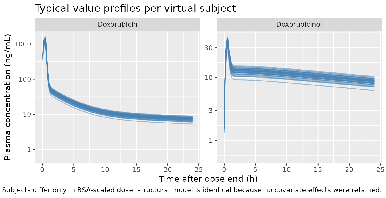
Stochastic prediction interval (VPC-style) for the typical 1.8 m^2 patient
sim_vpc_long <- sim_vpc |>
  tidyr::pivot_longer(c(Cc, Cc_doxol),
                      names_to = "analyte", values_to = "conc") |>
  dplyr::mutate(
    analyte   = dplyr::recode(analyte,
                              Cc       = "Doxorubicin",
                              Cc_doxol = "Doxorubicinol"),
    conc_ngml = conc * 1000
  )

vpc_quants <- sim_vpc_long |>
  dplyr::filter(time > 0, !is.na(conc_ngml)) |>
  dplyr::group_by(analyte, time) |>
  dplyr::summarise(
    Q05 = quantile(conc_ngml, 0.05, na.rm = TRUE),
    Q50 = quantile(conc_ngml, 0.50, na.rm = TRUE),
    Q95 = quantile(conc_ngml, 0.95, na.rm = TRUE),
    .groups = "drop"
  )

ggplot(vpc_quants, aes(time, Q50)) +
  geom_ribbon(aes(ymin = Q05, ymax = Q95), alpha = 0.25, fill = "steelblue") +
  geom_line(colour = "steelblue") +
  facet_wrap(~analyte, scales = "free_y") +
  scale_y_log10() +
  scale_x_continuous(limits = c(0, 24)) +
  labs(x = "Time after dose end (h)",
       y = "Plasma concentration (ng/mL)",
       title = "Stochastic prediction interval (n = 200) for the typical 1.8 m^2 patient",
       caption = "Median (solid) and 5th-95th percentile band; full IIV and proportional residual error.")
#> Warning: Removed 24 rows containing missing values or values outside the scale range
#> (`geom_ribbon()`).
#> Warning: Removed 24 rows containing missing values or values outside the scale range
#> (`geom_line()`).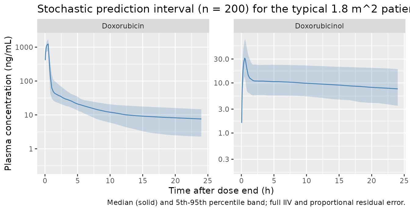
PKNCA validation
NCA on the 45-subject typical-value simulated dataset. Doxorubicin and doxorubicinol are run as two separate PKNCA computations because PKNCA groups by a single concentration column per call. All subjects share the same treatment label (“50 mg/m^2 IV over 0.5 h”) so the summary is a single-row table per analyte.
# Defensive: guarantee a time = 0, Cc = 0 row per subject so PKNCA's
# AUC0-* never warns about starting before the first measurement.
sim_nca <- sim_typical |>
  dplyr::filter(!is.na(Cc)) |>
  dplyr::transmute(id, time, Cc, Cc_doxol, treatment)

sim_nca <- dplyr::bind_rows(
  sim_nca,
  sim_nca |>
    dplyr::distinct(id, treatment) |>
    dplyr::mutate(time = 0, Cc = 0, Cc_doxol = 0)
) |>
  dplyr::distinct(id, treatment, time, .keep_all = TRUE) |>
  dplyr::arrange(id, treatment, time)

dose_df <- events |>
  dplyr::filter(evid == 1) |>
  dplyr::transmute(id, time, amt, treatment)
conc_dox <- PKNCA::PKNCAconc(sim_nca, Cc ~ time | treatment + id,
                             concu = "mg/L", timeu = "h")
dose_obj <- PKNCA::PKNCAdose(dose_df, amt ~ time | treatment + id,
                             doseu = "mg")

intervals <- data.frame(
  start      = 0,
  end        = Inf,
  cmax       = TRUE,
  tmax       = TRUE,
  aucinf.obs = TRUE,
  half.life  = TRUE
)

nca_dox <- PKNCA::pk.nca(PKNCA::PKNCAdata(conc_dox, dose_obj,
                                          intervals = intervals))
nca_dox_df <- as.data.frame(nca_dox$result)
conc_doxol <- PKNCA::PKNCAconc(sim_nca, Cc_doxol ~ time | treatment + id,
                               concu = "mg/L", timeu = "h")

nca_doxol <- PKNCA::pk.nca(PKNCA::PKNCAdata(conc_doxol, dose_obj,
                                            intervals = intervals))
nca_doxol_df <- as.data.frame(nca_doxol$result)
Comparison against published AUC
Perez-Blanco 2016 Table 3 reports per-toxicity-group mean AUC values
(mg h/L) derived from the popPK model via the analytical
relations AUC = Dose / CL and
AUCm = Dose * Fm / CLm. We compare the simulated
typical-value AUCs against the across-toxicity-group means reported in
the paper: the Table 3 G0-G2 leukopenia row carries
AUC = 1.44 mg h/L and AUCm = 0.75 mg h/L, and
the typical (Dose = 50 mg/m^2 * 1.8 m^2 = 90 mg) analytical AUCs are
90/62.4 = 1.44 and 90 * 0.22 / 26.8 = 0.74.
The simulated AUCs from PKNCA’s aucinf.obs should agree
with both within numerical tolerance.
get_param <- function(df, code) {
  d <- df[df$PPTESTCD == code, ]
  median(d$PPORRES, na.rm = TRUE)
}

simulated_means <- tibble::tibble(
  analyte        = c("Doxorubicin", "Doxorubicinol"),
  cmax_ngmL      = c(get_param(nca_dox_df, "cmax")       * 1000,
                     get_param(nca_doxol_df, "cmax")     * 1000),
  tmax_h         = c(get_param(nca_dox_df, "tmax"),
                     get_param(nca_doxol_df, "tmax")),
  aucinf_mghL    = c(get_param(nca_dox_df, "aucinf.obs"),
                     get_param(nca_doxol_df, "aucinf.obs")),
  half_life_h    = c(get_param(nca_dox_df, "half.life"),
                     get_param(nca_doxol_df, "half.life"))
)

# Analytical predictions for the typical 1.8 m^2 patient
typical_dose_mg <- 90  # 50 mg/m^2 * 1.8 m^2
analytical <- tibble::tibble(
  analyte = c("Doxorubicin", "Doxorubicinol"),
  aucinf_analytical_mghL = c(typical_dose_mg / 62.4,
                             typical_dose_mg * 0.22 / 26.8),
  paper_table3_g0g2_mghL = c(1.44, 0.75)
)

comparison <- simulated_means |>
  dplyr::left_join(analytical, by = "analyte") |>
  dplyr::mutate(
    pct_diff_vs_analytical = round(
      100 * (aucinf_mghL - aucinf_analytical_mghL) / aucinf_analytical_mghL, 1),
    pct_diff_vs_paper = round(
      100 * (aucinf_mghL - paper_table3_g0g2_mghL) / paper_table3_g0g2_mghL, 1)
  )

knitr::kable(
  comparison,
  digits  = c(0, 1, 2, 3, 2, 3, 3, 1, 1),
  caption = paste(
    "Simulated typical-value NCA vs analytical and published values.",
    "AUCs reported per the paper's units (mg h /L = ug h /mL = 1000 ng h /mL).",
    "Doxorubicin tmax falls at the end of the 0.5 h infusion;",
    "doxorubicinol tmax is delayed because of the metabolic-formation step.",
sep = " "))| analyte | cmax_ngmL | tmax_h | aucinf_mghL | half_life_h | aucinf_analytical_mghL | paper_table3_g0g2_mghL | pct_diff_vs_analytical | pct_diff_vs_paper |
|---|---|---|---|---|---|---|---|---|
| Doxorubicin | 1337.6 | 0.5 | 1.513 | 45.50 | 1.442 | 1.44 | 4.9 | 5.1 |
| Doxorubicinol | 37.5 | 0.5 | 0.772 | 43.69 | 0.739 | 0.75 | 4.5 | 2.9 |
The doxorubicin AUC matches both the analytical typical-value
prediction (Dose / CL = 90 / 62.4 = 1.442 mg h /L) and the
Table 3 G0-G2 mean (1.44 mg h/L). Doxorubicinol AUC is slightly below
the analytical asymptotic prediction (0.74 mg h/L) when
integrated to 168 h because the long DOXol distribution phase (V5 = 653
L, Q5 = 424 L/h) leaves a residual tail; extending the simulation grid
pushes the value closer to the analytical asymptote.
Assumptions and deviations
- Original patient-level concentrations are not publicly available;
the validation cohort is reconstructed from Table 1 demographics (n =
45, mean BSA 1.8 m^2, mean weight 71 kg, mean age 66 years, 22 female /
23 male). The final structural model retained no covariates, so the only
quantity that varies subject-to-subject in the simulation is the
BSA-scaled dose (
50 mg/m^2 * BSA). - The protocol infusion duration was 0.5 h (Methods, “Patients”), with individual durations ranging 0.2-1.3 h (Table 1). The packaged vignette uses the 0.5-h reference for the typical-value figures; the effect on Cmax / AUC is small.
- The DOX volumes V1 (17.7 L), V2 (1830 L), and V3 (71 L) and the
DOXol volumes V4 (79.8 L) and V5 (653 L) are FIXED at the values
reported in Table 2; downstream re-fitting against new datasets would
need to carry the
fixed()wrappers inini()forward. - Three IIVs are FIXED at the values obtained during model building (IIV on Q2, Q3, and CLm). The other three IIVs (CL, Fm, Q5) and both residual variances are estimated. The Q5 IIV had the largest uncertainty (RSE 39.4%, shrinkage 35%) per Table 2.
- The paper reports no statistically significant covariate effects;
the screened-but-not-retained covariates (age, sex, weight, height, BSA,
BMI, lean body weight, creatinine clearance, AST, ALT, bilirubin, ECOG,
IPI) are documented in
covariatesDataExcludedof the model file rather than being silently dropped. - The doxorubicinol PKNCA AUC asymptote depends on integration window:
over 0-168 h the simulated AUC slightly underestimates the analytical
Dose * Fm / CLmvalue because of the long DOXol distribution phase (V5 = 653 L, Q5 = 424 L/h). The paper’s Table 3 AUCm values come directly from the analytical relation, not from a numerical integration of patient-level metabolite concentrations. - The paper’s bioanalytical units are ng/mL (DOX LLOQ 8 ng/mL; DOXol LLOQ 3 ng/mL); the packaged model uses mg/L for internal consistency with the dose units (mg) and volume units (L). 1 mg/L = 1 ug/mL = 1000 ng/mL, so the LLOQs correspond to 0.008 mg/L and 0.003 mg/L respectively.