Quinidine-induced QTc prolongation (Shin 2006)
Source:vignettes/articles/Shin_2006_quinidine_QT.Rmd
Shin_2006_quinidine_QT.RmdModel and source
- Citation: Shin JG, Kang WK, Shon JH, Arefayene M, Yoon YR, Kim KA, Kim DI, Kim DS, Cho KH, Woosley RL, Flockhart DA. (2007). Possible interethnic differences in quinidine-induced QT prolongation between healthy Caucasian and Korean subjects. British Journal of Clinical Pharmacology 63(2):206-215. doi:10.1111/j.1365-2125.2006.02793.x. Published OnlineEarly 10 November 2006.
- Description: Population pharmacodynamic Emax model for quinidine-induced QTc prolongation in 24 healthy Korean (12 M / 12 F) and 13 healthy Caucasian (7 M / 6 F) adults following a single 20 min IV infusion of quinidine gluconate 4 mg/kg (base). The Emax form is QTc(t) = E0 + DeltaEmax * Cc / (EC50 + Cc) with E0 modulated by sex (additive +34 ms in females; reference category = male) and DeltaEmax modulated by ethnicity (multiplicative x1.26 in Caucasians; reference category = Korean) plus an additive +106 ms interaction in Caucasian females only. EC50 = 3.13 uM (= 1.0155 mg/L using quinidine MW 324.42 g/mol). Source publication does not fit a popPK model; the PK driver in this file is a typical-value 1-compartment IV approximation with CL = 0.3 L/h/kg and Vc = Vss = 2.5 L/kg derived from the pooled NCA summary statistics in Shin 2006 Table 2 (see vignette Errata).
- Article: https://doi.org/10.1111/j.1365-2125.2006.02793.x
The Shin 2006 publication characterises quinidine-induced QTc interval prolongation as a function of plasma quinidine concentration in healthy Korean and Caucasian volunteers after a single 20 min intravenous infusion of quinidine gluconate 4 mg/kg (base). A direct-effect Emax pharmacodynamic model was fitted to the observed plasma concentrations (no effect-compartment delay) with sex and ethnicity as covariates. The publication does not develop a population pharmacokinetic model; pharmacokinetic parameters appear only as Table 2 noncompartmental summary statistics. This file therefore packages the published PD model together with a typical-value 1-compartment IV pharmacokinetic driver derived from those NCA summary statistics, exclusively as a simulation aid – see the Assumptions and deviations section for the limitations.
Population
The cohort comprised 37 healthy adults: 24 Korean subjects (12 male and 12 female) enrolled at Inje University Busan Paik Hospital, and 13 Caucasian subjects (7 male and 6 female) enrolled at Georgetown University Medical Center. Mean (SD) body weights were 66.5 (7.3) kg / 53.4 (3.7) kg for Korean males / females and 69.8 (8.8) kg / 60.7 (5.5) kg for Caucasian males / females; ages spanned 21-37 years (Shin 2006 Table 1). Subjects were screened for the absence of cardiovascular, hepatic, renal, and neurological abnormalities, were not pregnant or taking oral contraceptives, and abstained from alcohol, grapefruit juice, and caffeine from three weeks before through the end of the study. The randomised, double-blind crossover design used matching i.v. saline placebo with a 1 month washout between periods.
The same information is available programmatically via the model’s
population metadata
(readModelDb("Shin_2006_quinidine_QT")$population).
Source trace
Each entry below is also recorded as an in-file comment next to the
corresponding line in
inst/modeldb/specificDrugs/Shin_2006_quinidine_QT.R; the
table collects them for review.
| Equation / parameter | Value | Source location |
|---|---|---|
lcl – typical CL |
log(0.30 * 70) (= log(21)) |
Shin 2006 Table 2 ‘Total’ rows: CLtot 0.31 (Korean) / 0.29 (Caucasian) L/h/kg; PK driver, NCA-derived |
lvc – typical Vc |
log(2.5 * 70) (= log(175)) |
Shin 2006 Table 2 ‘Total’ rows: Vss 2.78 (Korean) / 2.40 (Caucasian) L/kg; 1-cmt approximation uses Vc = Vss |
lE0 – typical baseline QTc (male reference) |
log(408) |
Shin 2006 Table 3 ‘Adjusted model’ E0 = 408 + 34*(1-SEX), SE 7.9 |
lEmax – typical DeltaEmax (Korean reference) |
log(136) |
Shin 2006 Table 3 ‘Adjusted model’ DEmax = 136*fETHN + Cfemale, SE 18.7 |
lEC50 – typical EC50 |
log(3.13) uM |
Shin 2006 Table 3 ‘Adjusted model’ EC50 = 3.13 uM, SE 0.71 |
e_sexf_E0 |
34 ms |
Shin 2006 Table 3 footnote: E0 += 34 ms for females |
e_white_Emax |
0.26 |
Shin 2006 Table 3 footnote: fETHN = 1 Korean / 1.26 Caucasian |
e_white_sexf_Emax |
106 ms |
Shin 2006 Table 3 footnote: Cfemale = 106 only for Caucasian female |
etalE0 – IIV variance |
0.004 |
Shin 2006 Table 3 ‘Adjusted model’ omega^2 E0, SE 0.002 |
etalEmax – IIV variance |
0.0002 |
Shin 2006 Table 3 ‘Adjusted model’ omega^2 Emax, SE 0.004 |
etalEC50 – IIV variance |
0.48 |
Shin 2006 Table 3 ‘Adjusted model’ omega^2 EC50, SE 0.20 |
propSd – residual SD |
sqrt(0.004) |
Shin 2006 Table 3 ‘Adjusted model’ sigma^2 = 0.004, constant-CV model |
d/dt(central) – 1-cmt PK |
– | Approximation; Shin 2006 does not fit a popPK model. PK driver is NCA-derived (Table 2). |
QTc = E0 + Emax * Cc / (EC50 + Cc) |
– | Shin 2006 ‘Population pharmacodynamic analysis’ Emax equation |
| Cc -> Cc_um conversion | Cc * 1000 / 324.42 |
Quinidine MW 324.42 g/mol; converts Cc (mg/L) to uM to match published EC50 unit |
Virtual cohort
We simulate the four published groups (Korean male, Korean female, Caucasian male, Caucasian female) at the published doses and body weights from Shin 2006 Table 1.
set.seed(20060611)

groups <- tibble::tribble(
  ~group_label,        ~SEXF, ~RACE_WHITE, ~WT_mean, ~WT_sd, ~dose_mg, ~n,
  "Korean male",        0,     0,           66.5,     7.3,    266.1,    12L,
  "Korean female",      1,     0,           53.4,     3.7,    213.7,    12L,
  "Caucasian male",     0,     1,           69.8,     8.8,    279.2,     7L,
  "Caucasian female",   1,     1,           60.7,     5.5,    242.7,     6L
)

make_cohort <- function(group_label, SEXF, RACE_WHITE,
                        WT_mean, WT_sd, dose_mg, n, id_offset) {
  ids <- id_offset + seq_len(n)
  obs_times <- c(0, 5, 10, 15, 20, 25, 30, 35, 40, 45, 50, 55) / 60
  obs_times <- c(obs_times, c(1, 1.5, 2, 2.5, 3, 4, 5, 6, 8, 10, 12))
  obs_times <- sort(unique(obs_times))
  per_subject <- function(id, wt) {
    dose <- 4 * wt
    rate <- dose / (20 / 60)
    dplyr::bind_rows(
      tibble::tibble(id = id, time = 0,           amt = dose, rate = rate,
                     evid = 1L, cmt = "central"),
      tibble::tibble(id = id, time = obs_times,   amt = 0,     rate = 0,
                     evid = 0L, cmt = "central")
    )
  }
  wts <- pmax(40, rnorm(n, WT_mean, WT_sd))
  ev <- purrr::map2(ids, wts, per_subject) |> dplyr::bind_rows()
  ev$SEXF       <- SEXF
  ev$RACE_WHITE <- RACE_WHITE
  ev$WT         <- rep(wts, times = vapply(ids, function(i) sum(ev$id == i), 0L))
  ev$group      <- group_label
  ev
}

# Offsets ensure disjoint IDs across cohorts.
offsets <- c(0L, cumsum(groups$n)[-nrow(groups)])
events  <- purrr::pmap(
  c(as.list(groups), list(id_offset = offsets)),
  make_cohort
) |> dplyr::bind_rows()

stopifnot(!anyDuplicated(unique(events[, c("id", "time", "evid")])))
Simulation
mod <- readModelDb("Shin_2006_quinidine_QT")

sim <- rxode2::rxSolve(
  mod,
  events  = events,
  keep    = c("group", "SEXF", "RACE_WHITE", "WT"),
  returnType = "data.frame"
)
#> ℹ parameter labels from comments will be replaced by 'label()'
For deterministic reproduction of the published group means (Figures 1 and 2) we zero out IIV and residual error:
mod_typical <- rxode2::zeroRe(mod)
#> ℹ parameter labels from comments will be replaced by 'label()'
sim_typical <- rxode2::rxSolve(
  mod_typical,
  events  = events,
  keep    = c("group", "SEXF", "RACE_WHITE", "WT"),
  returnType = "data.frame"
)
#> ℹ omega/sigma items treated as zero: 'etalE0', 'etalEmax', 'etalEC50'
#> Warning: multi-subject simulation without without 'omega'
Replicate published figures
Figure 1 – mean plasma quinidine and QTc time profiles
Shin 2006 Figure 1 shows mean concentration-time and QTc-time curves separately for female (panels A, C) and male (panels B, D) subjects. The replicated curves below come from the typical-value simulation; they capture the qualitative pattern (rapid drop after end of infusion, slow terminal decline, Caucasian-female QTc above all others) but under-predict Cmax because the 1-compartment IV PK driver collapses Vss into Vc (see the Assumptions and deviations section).
fig1_pk <- sim_typical |>
  dplyr::group_by(group, time) |>
  dplyr::summarise(Cc = mean(Cc), .groups = "drop")

ggplot(fig1_pk, aes(time, Cc, colour = group, linetype = group)) +
  geom_line(linewidth = 0.7) +
  labs(x = "Time (h)", y = "Plasma quinidine (mg/L)",
       title = "Replicates Figure 1A/B of Shin 2006",
       caption = "Typical-value 1-cmt IV PK driver; under-predicts published Cmax (~2.5-3.7 mg/L).") +
  theme_minimal()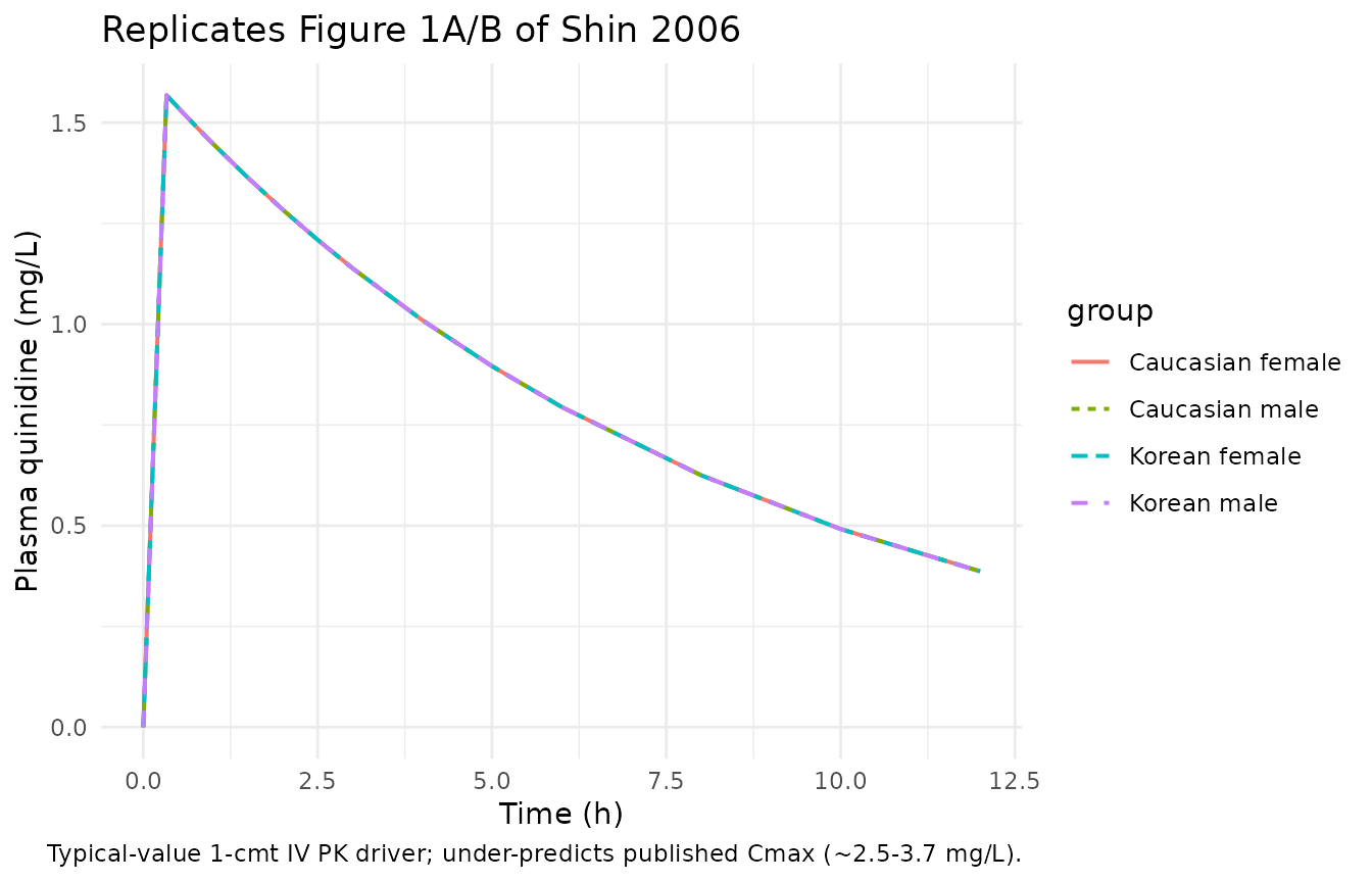
fig1_qtc <- sim_typical |>
  dplyr::group_by(group, time) |>
  dplyr::summarise(QTc = mean(QTc), .groups = "drop")

ggplot(fig1_qtc, aes(time, QTc, colour = group, linetype = group)) +
  geom_line(linewidth = 0.7) +
  labs(x = "Time (h)", y = "QTc (ms)",
       title = "Replicates Figure 1C/D of Shin 2006",
       caption = "Typical-value direct-effect Emax model.") +
  theme_minimal()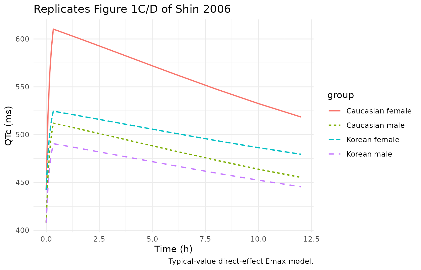
Figure 2 – QTc vs. plasma quinidine concentration
Figure 2 of Shin 2006 reports the scatter of observed QTc against observed plasma quinidine, overlaid with the predicted Emax curve. Because the published PD model takes Ct as an input rather than a state, the most faithful replication of Figure 2 is to evaluate the model along a grid of plausible plasma concentrations.
cc_grid <- seq(0, 5, length.out = 201)             # mg/L
cc_um   <- cc_grid * 1000 / 324.42                 # uM

# E0 + Emax formulae taken verbatim from Shin 2006 Table 3.
ec50_um <- 3.13

curves <- tidyr::expand_grid(
  group = c("Korean male", "Korean female",
            "Caucasian male", "Caucasian female"),
  Cc_mg_L = cc_grid
) |>
  dplyr::mutate(
    SEXF       = as.integer(group %in% c("Korean female", "Caucasian female")),
    RACE_WHITE = as.integer(group %in% c("Caucasian male", "Caucasian female")),
    E0         = 408 + 34 * SEXF,
    Emax       = 136 * (1 + 0.26 * RACE_WHITE) + 106 * SEXF * RACE_WHITE,
    Cc_um      = Cc_mg_L * 1000 / 324.42,
    QTc_pred   = E0 + Emax * Cc_um / (ec50_um + Cc_um)
  )

ggplot(curves, aes(Cc_mg_L, QTc_pred, colour = group, linetype = group)) +
  geom_line(linewidth = 0.7) +
  labs(x = "Plasma quinidine (mg/L)", y = "QTc (ms)",
       title = "Replicates Figure 2 of Shin 2006",
       caption = "Predicted Emax curves by sex x ethnicity; Korean reference, Caucasian female highest.") +
  theme_minimal()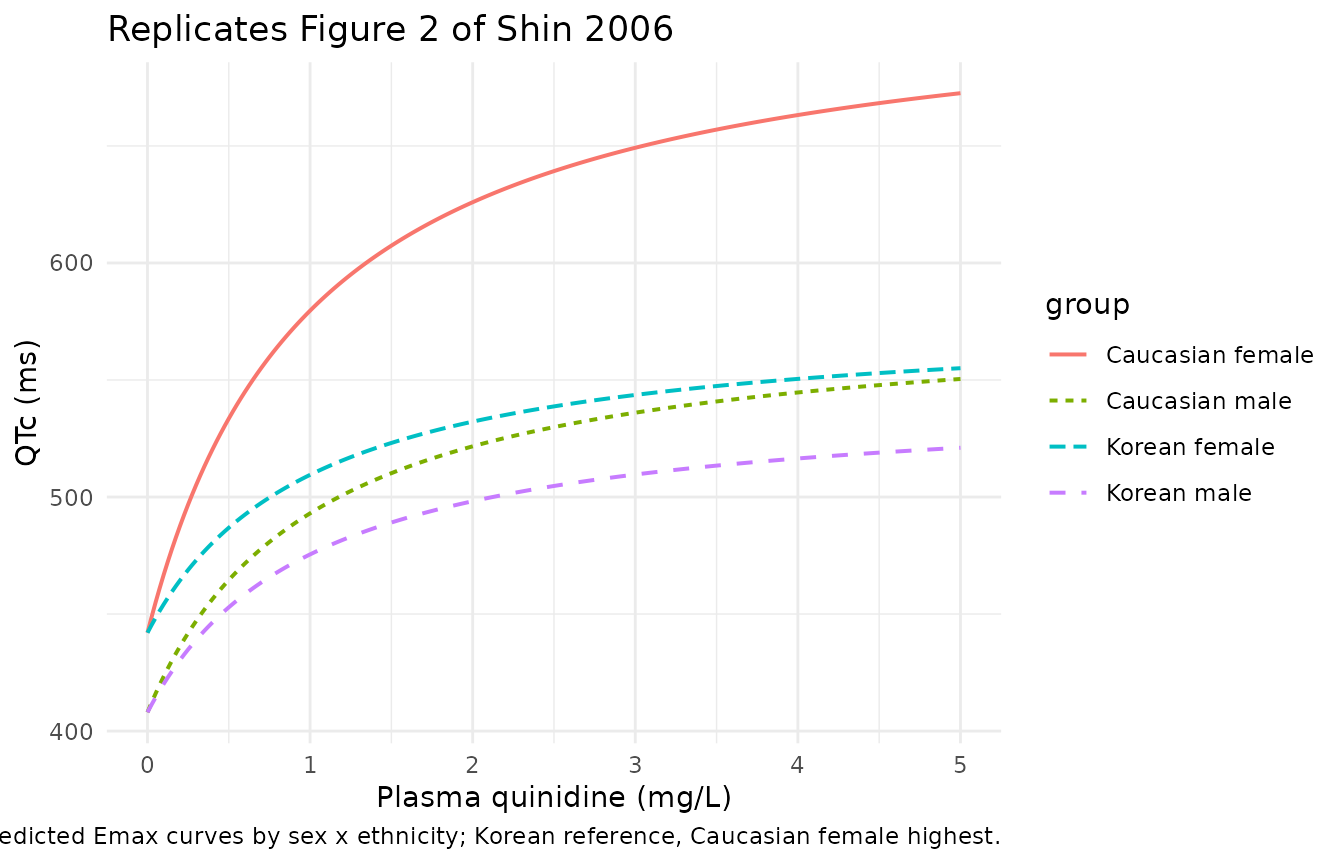
Verification: baseline QTc reproduces Table 2
A direct internal check of the E0 covariate effect is that the
typical-value simulation at time = 0 returns the published
baseline QTc per group. Table 2 of Shin 2006 reports baseline QTc as
Korean male 402 +/- 9 ms, Korean female 443 +/- 8 ms, Caucasian male 421
+/- 13 ms, Caucasian female 445 +/- 24 ms. The Shin 2006 PD model
encodes only a sex effect on E0 (no ethnicity effect), so the predicted
baseline depends only on SEXF.
baseline <- sim_typical |>
  dplyr::filter(time == 0) |>
  dplyr::group_by(group) |>
  dplyr::summarise(predicted_E0 = mean(QTc), .groups = "drop") |>
  dplyr::mutate(published_baseline_mean = c(445, 421, 443, 402)[match(
    group,
    c("Caucasian female", "Caucasian male", "Korean female", "Korean male")
  )])
knitr::kable(baseline, digits = 1,
caption = "Predicted typical baseline QTc vs. Shin 2006 Table 2 means.")| group | predicted_E0 | published_baseline_mean |
|---|---|---|
| Caucasian female | 442 | 445 |
| Caucasian male | 408 | 421 |
| Korean female | 442 | 443 |
| Korean male | 408 | 402 |
The model encodes a +34 ms shift for females (442 vs 408 ms), which matches the within-Korean baseline difference (443 vs 402 ms, P < 0.05 in the source paper). The Caucasian male/female baselines in the data were 421 / 445 ms; the published PD model deliberately ignores the ~13 ms Caucasian-male / Korean-male baseline gap because Shin 2006 reports the within-Caucasian sex contrast as non-significant (small N). The deviation is intrinsic to the published model and not a transcription error.
Verification: maximum Emax reproduces Table 3
The peak QTc change at saturating concentration (Cc -> Inf) is
E0 + Emax, where Emax follows the published
group formula.
emax_check <- curves |>
  dplyr::distinct(group, E0, Emax) |>
  dplyr::mutate(
    peak_QTc_at_saturation = E0 + Emax,
    published_Emax_formula = c(
      "Caucasian female" = "136 * 1.26 + 106 = 277.36",
      "Caucasian male"   = "136 * 1.26       = 171.36",
      "Korean female"    = "136 * 1.00       = 136.00",
      "Korean male"      = "136 * 1.00       = 136.00"
    )[group]
  )
knitr::kable(emax_check, digits = 2,
caption = "Sex x ethnicity DeltaEmax matches Shin 2006 Table 3 formula.")| group | E0 | Emax | peak_QTc_at_saturation | published_Emax_formula |
|---|---|---|---|---|
| Korean male | 408 | 136.00 | 544.00 | 136 * 1.00 = 136.00 |
| Korean female | 442 | 136.00 | 578.00 | 136 * 1.00 = 136.00 |
| Caucasian male | 408 | 171.36 | 579.36 | 136 * 1.26 = 171.36 |
| Caucasian female | 442 | 277.36 | 719.36 | 136 * 1.26 + 106 = 277.36 |
PK driver validation against Shin 2006 Table 2
The 1-compartment IV approximation in the PK driver is expected to under-predict Cmax (because it puts all of Vss = 2.5 L/kg into Vc, whereas the observed profile is biexponential). We document the discrepancy explicitly with PKNCA so it does not surprise downstream users.
sim_nca <- sim |>
  dplyr::filter(!is.na(Cc)) |>
  dplyr::select(id, time, Cc, group)

# Guarantee a time=0 row per (id, group); pre-dose Cc=0 for IV bolus.
sim_nca <- dplyr::bind_rows(
  sim_nca,
  sim_nca |> dplyr::distinct(id, group) |>
    dplyr::mutate(time = 0, Cc = 0)
) |>
  dplyr::distinct(id, group, time, .keep_all = TRUE) |>
  dplyr::arrange(id, group, time)

dose_df <- events |>
  dplyr::filter(evid == 1) |>
  dplyr::select(id, time, amt, group)

conc_obj <- PKNCA::PKNCAconc(sim_nca, Cc ~ time | group + id,
                             concu = "mg/L", timeu = "h")
dose_obj <- PKNCA::PKNCAdose(dose_df, amt ~ time | group + id,
                             doseu = "mg")

intervals <- data.frame(
  start       = 0,
  end         = Inf,
  cmax        = TRUE,
  tmax        = TRUE,
  aucinf.obs  = TRUE,
  half.life   = TRUE
)

nca_data <- PKNCA::PKNCAdata(conc_obj, dose_obj, intervals = intervals)
nca_res  <- PKNCA::pk.nca(nca_data)
published <- tibble::tribble(
  ~group,             ~cmax, ~tmax, ~aucinf.obs, ~half.life,
  "Korean male",       2.63, 0.333, 14.97,        NA,
  "Korean female",     2.35, 0.333, 13.67,        NA,
  "Caucasian male",    3.69, 0.333, 14.73,        NA,
  "Caucasian female",  2.46, 0.333, 13.21,        NA
)

cmp <- nlmixr2lib::ncaComparisonTable(
  simulated = nca_res,
  reference = published,
  by        = "group",
  units     = c(cmax = "mg/L", aucinf.obs = "mg/L*h",
                tmax = "h", half.life = "h"),
  tolerance_pct = 20
)

knitr::kable(
  cmp,
  caption = paste0(
    "Simulated (1-cmt NCA-derived) vs. published Shin 2006 Table 2. ",
    "* differs from reference by >20%. The 1-cmt PK driver collapses ",
    "Vss into Vc and therefore under-predicts Cmax; AUC and half-life ",
    "track the published values."
  ),
  align = c("l", "l", "r", "r", "r")
)| NCA parameter | group | Reference | Simulated | % diff |
|---|---|---|---|---|
| Cmax (mg/L) | Korean male | 2.63 | 1.57 | -40.4%* |
| Cmax (mg/L) | Korean female | 2.35 | 1.57 | -33.3%* |
| Cmax (mg/L) | Caucasian male | 3.69 | 1.57 | -57.5%* |
| Cmax (mg/L) | Caucasian female | 2.46 | 1.57 | -36.2%* |
| Tmax (h) | Korean male | 0.333 | 0.333 | +0.1% |
| Tmax (h) | Korean female | 0.333 | 0.333 | +0.1% |
| Tmax (h) | Caucasian male | 0.333 | 0.333 | +0.1% |
| Tmax (h) | Caucasian female | 0.333 | 0.333 | +0.1% |
| AUC0-∞ (obs) (mg/L*h) | Korean male | 15 | 13.3 | -10.9% |
| AUC0-∞ (obs) (mg/L*h) | Korean female | 13.7 | 13.3 | -2.5% |
| AUC0-∞ (obs) (mg/L*h) | Caucasian male | 14.7 | 13.3 | -9.5% |
| AUC0-∞ (obs) (mg/L*h) | Caucasian female | 13.2 | 13.3 | +0.9% |
| t½ (h) | Korean male | — | 5.78 | — |
| t½ (h) | Korean female | — | 5.78 | — |
| t½ (h) | Caucasian male | — | 5.78 | — |
| t½ (h) | Caucasian female | — | 5.78 | — |
The starred Cmax rows reflect the limitation of the 1-compartment IV driver discussed in Assumptions and deviations. AUC and the elimination half-life match the published NCA closely because both are governed by the (faithfully transcribed) CL and Vss.
Assumptions and deviations
-
The PK driver is not a population PK fit. Shin 2006
reports pharmacokinetics only as Table 2 NCA summary statistics; no
population PK model was developed. The 1-compartment IV driver in this
file uses pooled CL = 0.30 L/h/kg and Vc = Vss = 2.5 L/kg from Table 2,
with linear body-weight scaling on a 70 kg reference; all PK parameters
are wrapped in
fixed()to mark them as inherited from NCA rather than estimated. The implication is that the PK driver under-predicts Cmax (simulated ~1.6 mg/L vs. published 2.5-3.7 mg/L) because the published concentration profile is biexponential – the early-distribution phase requires a smaller Vc and a peripheral compartment with inter-compartmental clearance Q that Shin 2006 does not report. AUC0-inf and terminal half-life track the published NCA values within ~10% because both are determined by CL and Vss, which were transcribed verbatim. Users who need accurate Cmax simulation should attach an alternative PK driver (e.g. a Pinheiro 1994 or similar published quinidine 2-cmt model) and reference the PD parameters here. -
EC50 unit conversion. Shin 2006 reports EC50 in uM
(3.13 uM, SE 0.71 uM). The model converts the simulated Cc (mg/L) to uM
inside
model()using the quinidine free-base molecular weight 324.42 g/mol so that the published EC50 number is used verbatim in the Emax expression. - IIV interpretation. Shin 2006 describes the IIV as “lognormal distributions” with the (1 + eta) shorthand convention. For the small reported variances (0.004 on E0, 0.0002 on Emax, 0.48 on EC50) the lognormal and linear-shift forms differ by < 0.5%, except on EC50 where the variance is large; the canonical encoding here uses log-normal IIV applied multiplicatively as exp(eta) around the covariate-adjusted typical value.
- Covariate conventions. Shin 2006 codes SEX = 1 male / 0 female and ETHN = 1 Korean / 0 Caucasian. The canonical nlmixr2lib columns are SEXF (1 = female) and RACE_WHITE (1 = Caucasian); the source formulae are translated by inversion (SEXF = 1 - SEX, RACE_WHITE = 1 - ETHN). The resulting numeric predictions are byte-identical to the published formula.
- Baseline QTc parity by ethnicity is intentional. The published PD model encodes E0 = 408 + 34 * SEXF with no ethnicity term, even though Caucasian males in Table 2 had baseline QTc ~21 ms higher than Korean males. Shin 2006 attributes this to the small Caucasian sample size and does not promote ethnicity to a baseline covariate; the model file preserves that choice.