Model and source
- Citation: Kim YK, Jo KM, Lee JH, Jang JH, Choe EJ, Kang G, Zang DY, Lee DH. Beyond One-Size-Fits-All: Tailoring Teicoplanin Regimens for Normal Renal Function Patients Using Population Pharmacokinetics and Monte Carlo Simulation. Pharmaceutics. 2024;16(4):499. doi:10.3390/pharmaceutics16040499
- Description: Three-compartment population PK model for intravenous teicoplanin in healthy Korean adults with normal renal function, with a power effect of BSA-adjusted CKD-EPI creatinine eGFR on total clearance and a power effect of body weight on the second peripheral volume (Kim 2024)
- Article: https://doi.org/10.3390/pharmaceutics16040499
- PMC record: https://www.ncbi.nlm.nih.gov/pmc/articles/PMC11053983/
Kim and colleagues gave a single 200 mg intravenous dose of teicoplanin, infused over 30 minutes, to 12 healthy Korean adults and described the resulting plasma concentrations with a three-compartment model fitted in NONMEM 7.5 (FOCE-I). The estimated glomerular filtration rate from the CKD-EPI creatinine equation, de-normalized to each subject’s body surface area, was retained as a power covariate on total clearance, and body weight as a power covariate on the second peripheral volume. The fitted model was then used for Monte Carlo dosing simulations in patients with normal renal function.
Population
Twelve healthy adults (6 female, 6 male) aged 19-55 years by protocol, with a median age of 32.0 years (IQR 30.0-40.3), median weight 67.9 kg (IQR 51.3-73.4), median height 164 cm (IQR 158-169) and median body surface area 1.77 m^2 (IQR 1.52-1.85) contributed 96 plasma concentrations (Kim 2024 Table 1, Section 3.1). Renal function was normal throughout: median serum creatinine 0.875 mg/dL, median cystatin C 0.760 mg/dL, and a median BSA-adjusted CKD-EPI creatinine eGFR of 105 mL/min (IQR 96.7-113).
Each subject was sampled eight times after the start of the infusion: at 33, 36, 45 and 90 minutes, at 4 and 8 hours, once in a 48-120 hour window and once in a 168-240 hour window (Kim 2024 Section 2.2). This sparse terminal sampling is important for the validation below - the paper’s own noncompartmental analysis is a grid-limited view of a model whose true terminal half-life is roughly twice the half-life the NCA recovers.
The same information is available programmatically via the model’s
population metadata
(readModelDb("Kim_2024_teicoplanin")()$population).
Source trace
The per-parameter origin is recorded as an in-file comment next to
each ini() entry in
inst/modeldb/specificDrugs/Kim_2024_teicoplanin.R. The
table below collects them in one place for review.
| Equation / parameter | Value | Source location |
|---|---|---|
CL = theta1 * (CE/105.27)^theta2 |
n/a | Kim 2024 Table 2, “Structural model” |
lcl (theta1) |
0.693 L/h | Kim 2024 Table 2 (RSE 2.97%; bootstrap 0.693, 95% CI 0.653-0.74) |
e_crcl_cl (theta2) |
0.785 | Kim 2024 Table 2 (RSE 16.2%; bootstrap 0.789, 95% CI 0.422-1.16) |
lvc (theta3, V1) |
3.96 L | Kim 2024 Table 2 (RSE 8.41%; bootstrap 3.97, 95% CI 3.15-4.62) |
lq (theta4, Q2) |
4.45 L/h | Kim 2024 Table 2 (RSE 11.6%; bootstrap 4.45, 95% CI 3.63-5.86) |
lvp (theta5, V2) |
8.24 L | Kim 2024 Table 2 (RSE 8.32%; bootstrap 8.33, 95% CI 7.07-9.85) |
lq2 (theta6, Q3) |
1.76 L/h | Kim 2024 Table 2 (RSE 9.7%; bootstrap 1.75, 95% CI 1.44-2.13) |
V3 = theta7 * (WT/67.85)^theta8 |
n/a | Kim 2024 Table 2, “Structural model” |
lvp2 (theta7) |
69.8 L | Kim 2024 Table 2 (RSE 8.74%; bootstrap 69.7, 95% CI 55.8-82.6) |
e_wt_vp2 (theta8) |
1.73 | Kim 2024 Table 2 (RSE 22.6%; bootstrap 1.73, 95% CI 0.67-2.44) |
etalcl |
8.83% CV, fixed | Kim 2024 Table 2, “Interindividual variability”; superscript
f
|
etalvc |
23.8% CV, fixed | Kim 2024 Table 2; superscript f
|
etalq |
32.7% CV | Kim 2024 Table 2 (RSE 20.2%; bootstrap 30.7, 95% CI 14.2-42.2) |
etalvp |
23.9% CV, fixed | Kim 2024 Table 2; superscript f
|
etalq2 |
31.0% CV | Kim 2024 Table 2 (RSE 18.9%; bootstrap 29.6, 95% CI 16.7-41.4) |
etalvp2 |
7.54% CV, fixed | Kim 2024 Table 2; superscript f
|
propSd |
6.33% | Kim 2024 Table 2, “Residual variability” (RSE 13.1%; bootstrap 6.22, 95% CI 4.63-7.94) |
Covariate CRCL definition |
n/a | Kim 2024 Table 2 footnote (CE) and Table 1 footnotes c,
e |
Covariate WT reference 67.85 kg |
n/a | Kim 2024 Table 2, “Structural model” (cohort median weight, Table 1) |
| Three-compartment IV structure | n/a | Kim 2024 Section 3.2 (NONMEM ADVAN11 TRANS4) |
| 30-minute IV infusion, 200 mg | n/a | Kim 2024 Section 2.2 |
The IIV percentages are converted to the internal log-normal variance
scale with omega^2 = log(1 + CV^2); each converted value
appears as an in-file comment on the corresponding ini()
line.
Structural check against the paper’s derived quantities
Before any simulation, the packaged ini() values are
checked against three quantities the paper reports separately
from Table 2, so a mis-transcribed theta shows up immediately. All
inputs below come from the model object; all targets come from the
paper.
ui <- rxode2::rxode(readModelDb("Kim_2024_teicoplanin"))
#> ℹ parameter labels from comments will be replaced by 'label()'
th <- ui$theta

cl_typ  <- exp(th[["lcl"]])
vc_typ  <- exp(th[["lvc"]])
q_typ   <- exp(th[["lq"]])
vp_typ  <- exp(th[["lvp"]])
q2_typ  <- exp(th[["lq2"]])
vp2_typ <- exp(th[["lvp2"]])
vss_typ <- vc_typ + vp_typ + vp2_typ

# Micro-constants and the three macro half-lives (eigenvalues of the
# three-compartment rate matrix).
k10 <- cl_typ / vc_typ; k12 <- q_typ / vc_typ; k21 <- q_typ / vp_typ
k13 <- q2_typ / vc_typ; k31 <- q2_typ / vp2_typ
rate_matrix <- matrix(
  c(-(k10 + k12 + k13), k21,  k31,
    k12,                -k21, 0,
    k13,                0,    -k31),
  nrow = 3, byrow = TRUE
)
half_lives <- sort(log(2) / -Re(eigen(rate_matrix)$values))

structural <- tibble::tribble(
  ~Quantity,                      ~Model,        ~Published, ~Source,
  "Typical CL (L/h)",             cl_typ,        0.693,      "Kim 2024 Section 4 ('typical values of CL ... 0.693 L/h')",
  "Typical Vss = V1+V2+V3 (L)",   vss_typ,       82.0,       "Kim 2024 Section 4 ('... and 82.0 L')",
  "1st half-life (h)",            half_lives[1], 0.345,      "Kim 2024 Table 3, mean 1st t1/2",
  "2nd half-life (h)",            half_lives[2], 4.12,       "Kim 2024 Table 3, mean 2nd t1/2",
  "3rd half-life (h)",            half_lives[3], 103,        "Kim 2024 Table 3, mean 3rd t1/2"
) |>
  dplyr::mutate(`% diff` = 100 * (Model - Published) / Published)

structural |>
  dplyr::select(Quantity, Model, Published, `% diff`, Source) |>
  knitr::kable(digits = c(0, 4, 3, 2, 0),
caption = "Model-derived structural quantities vs. values Kim 2024 reports outside Table 2.")| Quantity | Model | Published | % diff | Source |
|---|---|---|---|---|
| Typical CL (L/h) | 0.6930 | 0.693 | 0.00 | Kim 2024 Section 4 (‘typical values of CL … 0.693 L/h’) |
| Typical Vss = V1+V2+V3 (L) | 82.0000 | 82.000 | 0.00 | Kim 2024 Section 4 (‘… and 82.0 L’) |
| 1st half-life (h) | 0.3254 | 0.345 | -5.68 | Kim 2024 Table 3, mean 1st t1/2 |
| 2nd half-life (h) | 4.0353 | 4.120 | -2.06 | Kim 2024 Table 3, mean 2nd t1/2 |
| 3rd half-life (h) | 106.4298 | 103.000 | 3.33 | Kim 2024 Table 3, mean 3rd t1/2 |
# CL and Vss are stated to three significant figures in the Discussion, so they
# must agree essentially exactly; the half-lives are compared against the MEAN of
# 12 individual post-hoc values, which is not the typical-value quantity, so a
# looser bound applies there. Both are deterministic (no simulation, no RNG).
stopifnot(
  abs(structural$`% diff`[structural$Quantity == "Typical CL (L/h)"]) < 0.5,
  abs(structural$`% diff`[structural$Quantity == "Typical Vss = V1+V2+V3 (L)"]) < 0.5,
  max(abs(structural$`% diff`[grepl("half-life", structural$Quantity)])) < 15
)
The third half-life is the point of the paper’s own caution: the model’s terminal half-life is roughly 106 h, while the noncompartmental terminal half-life the same data support is only about 55 h (Kim 2024 Table 3, Section 3.3). Both are reproduced below.
Virtual cohort
Original observed data are not publicly available. The cohort below draws body weight and BSA-adjusted CKD-EPI creatinine eGFR from log-normal distributions matched to the mean and CV% reported in Kim 2024 Table 1, and samples each subject at the paper’s own eight measurement times.
# `set.seed()` seeds R's RNG (the covariate draws). It does NOT seed rxode2's
# simulation RNG, whose streams are partitioned per solver thread -- so the
# realised etas differ between a 2-core CI runner and a 16-thread workstation.
# Every assertion below is written to hold for any cohort the model can produce.
set.seed(20240405)
rxode2::rxSetSeed(20240405)

n_subj <- 200L

# Log-normal parameters from a mean and a CV%.
lnorm_pars <- function(mean_val, cv) {
  sdlog <- sqrt(log(1 + cv^2))
  list(meanlog = log(mean_val) - sdlog^2 / 2, sdlog = sdlog)
}
wt_p   <- lnorm_pars(64.8, 0.199)   # Kim 2024 Table 1, weight
crcl_p <- lnorm_pars(103,  0.155)   # Kim 2024 Table 1, adjusted eGFR by CKD-EPI CR for BSA

subjects <- tibble(
  id        = seq_len(n_subj),
  WT        = rlnorm(n_subj, wt_p$meanlog,   wt_p$sdlog),
  CRCL      = rlnorm(n_subj, crcl_p$meanlog, crcl_p$sdlog),
  treatment = "200 mg IV, 30-min infusion"
)

# The paper's eight sampling times (Kim 2024 Section 2.2). The 48-120 h and
# 168-240 h windows are represented by 84 h (the window midpoint) and 192 h
# (the reported median Tlast, Table 3).
paper_times <- c(33 / 60, 36 / 60, 45 / 60, 90 / 60, 4, 8, 84, 192)

# A denser grid for the profile figure; the NCA below is restricted to
# `paper_times` so it reproduces the paper's measurement grid rather than
# improving on it.
dense_times <- sort(unique(c(
  0, paper_times,
  seq(0.05, 2, by = 0.05), seq(2.5, 12, by = 0.5), seq(14, 240, by = 2)
)))

doses <- subjects |>
  mutate(time = 0, amt = 200, dur = 0.5, evid = 1L, cmt = "central")

obs <- subjects |>
  tidyr::crossing(time = dense_times) |>
  mutate(amt = NA_real_, dur = NA_real_, evid = 0L, cmt = "central")

events <- bind_rows(doses, obs) |> arrange(id, time, desc(evid))
stopifnot(!anyDuplicated(unique(events[, c("id", "time", "evid")])))
Simulation
mod <- readModelDb("Kim_2024_teicoplanin")
sim <- rxode2::rxSolve(mod, events = events,
                       keep = c("WT", "CRCL", "treatment")) |>
  as.data.frame()
#> ℹ parameter labels from comments will be replaced by 'label()'

# Solver sanity: concentrations must be positive everywhere on the grid, or the
# log-scale figure and PKNCA's terminal-slope fit are both meaningless.
stopifnot(all(sim$Cc[sim$time > 0] > 0), !anyNA(sim$Cc))
Terminal half-life of the solved system
The eigenvalue half-life computed above is an algebraic property of
the ini() values. Fitting the terminal slope of the
solved profile checks that the ODE block is wired consistently
with those values.
mod_typical <- mod |> rxode2::zeroRe()
#> ℹ parameter labels from comments will be replaced by 'label()'
long_ev <- rxode2::et(amt = 200, dur = 0.5, cmt = "central") |>
  rxode2::et(seq(0, 1500, by = 5))
sim_typ <- rxode2::rxSolve(
  mod_typical, events = long_ev,
  params = c(WT = 67.85, CRCL = 105.27)
) |>
  as.data.frame()
#> ℹ omega/sigma items treated as zero: 'etalcl', 'etalvc', 'etalq', 'etalvp', 'etalq2', 'etalvp2'

# Keep Cc >= 1e-6 * max(Cc): below that the ODE solution is integrator noise.
tail_fit <- sim_typ |> dplyr::filter(time >= 800, time <= 1500, Cc >= 1e-6 * max(Cc))
slope_hl <- log(2) / -stats::coef(stats::lm(log(Cc) ~ time, data = tail_fit))[["time"]]

cat(sprintf("Eigenvalue t1/2 = %.2f h; solved terminal-slope t1/2 = %.2f h (%.2f%% diff)\n",
            half_lives[3], slope_hl, 100 * (slope_hl - half_lives[3]) / half_lives[3]))
#> Eigenvalue t1/2 = 106.43 h; solved terminal-slope t1/2 = 106.43 h (0.00% diff)

# Deterministic (zeroRe + fixed covariates), so a tight bound is correct here.
stopifnot(abs(slope_hl - half_lives[3]) / half_lives[3] < 0.02)
Replicate published figures
sim |>
  dplyr::filter(time > 0) |>
  group_by(time) |>
  summarise(
    Q10 = quantile(Cc, 0.10),
    Q50 = quantile(Cc, 0.50),
    Q90 = quantile(Cc, 0.90),
    .groups = "drop"
  ) |>
  ggplot(aes(time, Q50)) +
  geom_ribbon(aes(ymin = Q10, ymax = Q90), alpha = 0.25) +
  geom_line() +
  geom_vline(xintercept = paper_times, linetype = "dotted", colour = "grey40") +
  scale_x_continuous(breaks = c(0, 24, 48, 96, 144, 192, 240)) +
  scale_y_log10() +
  labs(x = "Time (h)", y = "Teicoplanin concentration (mg/L)",
       title = "Single 200 mg IV infusion - median with 10th-90th percentiles",
       caption = "Dotted lines mark the paper's eight sampling times (Kim 2024 Section 2.2).")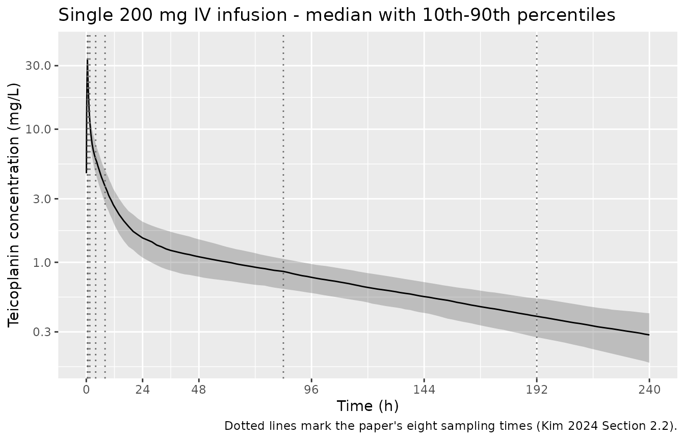
Simulated concentration-time profile after a single 200 mg 30-minute IV infusion. Replicates the shape of Figure S2 of Kim 2024 (visual predictive check, 0-240 h).
PKNCA validation
The NCA below deliberately uses only the paper’s eight sampling times. A denser grid would estimate the model’s true terminal phase and would move the half-life, Vz and Vss away from the paper’s published NCA, which was computed from those eight points.
sim_nca <- sim |>
  dplyr::filter(!is.na(Cc), time %in% c(0, paper_times)) |>
  dplyr::select(id, time, Cc, treatment, WT)

# Guarantee a time = 0 row per subject (pre-dose concentration is 0).
sim_nca <- dplyr::bind_rows(
  sim_nca,
  sim_nca |> dplyr::distinct(id, treatment, WT) |>
    dplyr::mutate(time = 0, Cc = 0)
) |>
  dplyr::distinct(id, treatment, time, .keep_all = TRUE) |>
  dplyr::arrange(id, treatment, time)

stopifnot(nrow(sim_nca) == n_subj * (length(paper_times) + 1L))

conc_obj <- PKNCA::PKNCAconc(sim_nca, Cc ~ time | treatment + id,
                             concu = "mg/L", timeu = "h")

dose_df <- events |>
  dplyr::filter(evid == 1) |>
  dplyr::select(id, time, amt, treatment)
dose_obj <- PKNCA::PKNCAdose(dose_df, amt ~ time | treatment + id, doseu = "mg")

intervals <- data.frame(
  start       = 0,
  end         = Inf,
  cmax        = TRUE,
  clast.obs   = TRUE,
  auclast     = TRUE,
  aucinf.obs  = TRUE,
  aumclast    = TRUE,
  aumcinf.obs = TRUE,
  mrt.obs     = TRUE,
  half.life   = TRUE,
  cl.obs      = TRUE,
  vz.obs      = TRUE,
  vss.obs     = TRUE
)

nca_res <- PKNCA::pk.nca(PKNCA::PKNCAdata(conc_obj, dose_obj, intervals = intervals))
Kim 2024 reports the terminal slope as having been fitted from three or four points per subject (“four concentration measurements were taken for nine subjects and three for the remaining three subjects”, Section 3.3). PKNCA’s automatic window selection on the same grid should land in the same place.
lz_n <- as.data.frame(nca_res$result) |>
  dplyr::filter(PPTESTCD == "lambda.z.n.points")
print(table(`Points in the terminal fit` = lz_n$PPORRES))
#> Points in the terminal fit
#>   3   4   5
#>  81 101  18

# PKNCA's automatic window occasionally reaches back to the 1.5 h sample and
# takes a fifth point, which the paper's manual fit did not; that is a handful
# of subjects, not the typical behaviour. Gate the median (robust to which
# subjects land in the tail) and a generous floor on the 3-or-4 fraction
# (realised ~0.94; MC-SE ~1.7 percentage points at 200 subjects). A denser
# terminal grid would push this well past 5 points and break both bounds.
stopifnot(
  median(lz_n$PPORRES) %in% c(3, 4),
  mean(lz_n$PPORRES %in% c(3, 4)) > 0.8
)
Comparison against published NCA
Kim 2024 Table 3 reports both a mean (CV%) and a median (IQR) for
every NCA parameter. ncaComparisonTable() pools the
simulated side by median, so the published medians are
the like-for-like reference. Clearance and the two volumes are published
per kilogram, so the simulated values are divided by each subject’s
weight before the comparison.
sim_result <- as.data.frame(nca_res$result) |>
  dplyr::left_join(subjects |> dplyr::select(id, WT), by = "id") |>
  dplyr::mutate(
    PPORRES = dplyr::if_else(
      PPTESTCD %in% c("cl.obs", "vz.obs", "vss.obs"),
      PPORRES / WT,
      PPORRES
    )
  ) |>
  dplyr::select(-WT)

published <- tibble::tribble(
  ~treatment,                   ~cmax, ~clast.obs, ~auclast, ~aucinf.obs, ~aumclast, ~aumcinf.obs, ~mrt.obs, ~half.life, ~cl.obs, ~vz.obs, ~vss.obs,
  "200 mg IV, 30-min infusion", 30.9,  0.422,      270,      305,         13800,     22300,        76.7,     55.0,       0.0103,  0.761,   0.734
)

cmp <- nlmixr2lib::ncaComparisonTable(
  simulated     = sim_result,
  reference     = published,
  by            = "treatment",
  units         = c(cmax = "mg/L", clast.obs = "mg/L", auclast = "mg/L*h",
                    aucinf.obs = "mg/L*h", aumclast = "mg/L*h^2",
                    aumcinf.obs = "mg/L*h^2", mrt.obs = "h", half.life = "h",
                    cl.obs = "L/h/kg", vz.obs = "L/kg", vss.obs = "L/kg"),
  tolerance_pct = 20
)

knitr::kable(
  cmp,
  caption = "Simulated (median of 200 virtual subjects, paper's sampling grid) vs. Kim 2024 Table 3 medians. * differs from reference by >20%.",
  align = c("l", "l", "r", "r", "r")
)| NCA parameter | treatment | Reference | Simulated | % diff |
|---|---|---|---|---|
| Cmax (mg/L) | 200 mg IV, 30-min infusion | 30.9 | 30.7 | -0.6% |
| Clast (mg/L) | 200 mg IV, 30-min infusion | 0.422 | 0.407 | -3.5% |
| AUC0-∞ (obs) (mg/L*h) | 200 mg IV, 30-min infusion | 305 | 313 | +2.6% |
| AUClast (mg/L*h) | 200 mg IV, 30-min infusion | 270 | 277 | +2.5% |
| t½ (h) | 200 mg IV, 30-min infusion | 55 | 53.3 | -3.1% |
| CL/F (L/h/kg) | 200 mg IV, 30-min infusion | 0.0103 | 0.00987 | -4.2% |
| Vss/F (L/kg) | 200 mg IV, 30-min infusion | 0.734 | 0.76 | +3.5% |
| MRT (h) | 200 mg IV, 30-min infusion | 76.7 | 73.4 | -4.3% |
| Vz/F (L/kg) | 200 mg IV, 30-min infusion | 0.761 | 0.813 | +6.8% |
| AUMC0-∞ (obs) (mg/L*h^2) | 200 mg IV, 30-min infusion | 22300 | 22400 | +0.5% |
| AUMC0-t (mg/L*h^2) | 200 mg IV, 30-min infusion | 13800 | 14200 | +2.9% |
# Structural gate. A mis-transcribed clearance, volume, dose or unit moves the
# whole distribution by tens of percent; the residual disagreement here is the
# difference between a 200-subject log-normal covariate cohort and the paper's
# 12 actual subjects, which is a few percent on every parameter. The bound is
# the tolerance_pct the table itself is starred at.
pct <- suppressWarnings(as.numeric(gsub("[^0-9.eE+-]", "", cmp$`% diff`)))
stopifnot(!anyNA(pct), max(abs(pct)) < 20)
ncaComparisonTable() takes the apparent-clearance labels
CL/F, Vz/F and Vss/F from
nlmixr2lib::ncaParamLabel(). Teicoplanin was given
intravenously here, so bioavailability is 1 by construction and those
rows are the absolute CL, Vz and
Vss per kilogram that Kim 2024 Table 3 reports.
The NCA half-life is not the model’s terminal half-life
Kim 2024 flags this explicitly: “The values for t1/2 lambda z significantly diverged from the three half-lives obtained through population PK analysis”, and “the steady-state volume of distribution from NCA (VssNCA) significantly differed from that determined by population PK (VSS)” (Section 3.3). Reproducing both sides of that discrepancy is a stronger check on the model than matching either one alone.
sim_par <- sim |>
  dplyr::distinct(id, .keep_all = TRUE) |>
  dplyr::mutate(vss_i = (vc + vp + vp2) / WT, cl_i = cl / WT, vc_i = vc / WT,
                auc_i = 200 / cl)

nca_med <- function(code) {
  median(sim_result$PPORRES[sim_result$PPTESTCD == code], na.rm = TRUE)
}

discrepancy <- tibble::tribble(
  ~Quantity,                    ~`NCA (sparse grid)`, ~`Population PK`, ~`Published NCA`, ~`Published popPK`,
  "Vss (L/kg)",                 nca_med("vss.obs"),   median(sim_par$vss_i), 0.734,        1.24,
  "Terminal half-life (h)",     nca_med("half.life"), half_lives[3],         55.0,         97.9,
  "CL (L/h/kg)",                nca_med("cl.obs"),    median(sim_par$cl_i),  0.0103,       0.0104
)

knitr::kable(discrepancy, digits = 4,
caption = "Kim 2024 Table 3: NCA and population-PK views of the same subjects. Published columns are the Table 3 medians.")| Quantity | NCA (sparse grid) | Population PK | Published NCA | Published popPK |
|---|---|---|---|---|
| Vss (L/kg) | 0.7596 | 1.1841 | 0.7340 | 1.2400 |
| Terminal half-life (h) | 53.2843 | 106.4298 | 55.0000 | 97.9000 |
| CL (L/h/kg) | 0.0099 | 0.0106 | 0.0103 | 0.0104 |
# The NCA/popPK Vss ratio and half-life ratio are the paper's own observation.
# Published: Vss 0.734 vs 1.24 (ratio 0.59); t1/2 55.0 vs 97.9 (ratio 0.56).
stopifnot(
  abs(nca_med("vss.obs") / median(sim_par$vss_i) - 0.734 / 1.24) < 0.10,
  abs(nca_med("half.life") / half_lives[3] - 55.0 / 97.9) < 0.10
)
The population-PK column of Kim 2024 Table 3 is also reproduced directly.
poppk <- tibble::tribble(
  ~Quantity,        ~Model, ~Published,
  "CL (L/h/kg)",    median(sim_par$cl_i),  0.0104,
  "Vc (L/kg)",      median(sim_par$vc_i),  0.0649,
  "Vss (L/kg)",     median(sim_par$vss_i), 1.24,
  "AUC (mg/L*h)",   median(sim_par$auc_i), 300
) |>
  dplyr::mutate(`% diff` = 100 * (Model - Published) / Published)

knitr::kable(poppk, digits = c(0, 5, 4, 1),
caption = "Individual population-PK parameters: simulated medians vs. Kim 2024 Table 3 'Population PK results' medians.")| Quantity | Model | Published | % diff |
|---|---|---|---|
| CL (L/h/kg) | 0.01064 | 0.0104 | 2.3 |
| Vc (L/kg) | 0.06149 | 0.0649 | -5.3 |
| Vss (L/kg) | 1.18408 | 1.2400 | -4.5 |
| AUC (mg/L*h) | 301.79669 | 300.0000 | 0.6 |
Dosing simulations (Figures 2 and 4)
Kim 2024 used the model to recommend regimens for patients with normal renal function: a loading dose every 12 h for four doses, then a maintenance dose every 24 h. Troughs are read just before each dose on days 3 to 7. Three of the paper’s stated results are reproduced below.
make_regimen <- function(ld_mgkg, md_mgkg, label, id_offset, seed) {
  set.seed(seed)
  s <- tibble(
    id      = id_offset + seq_len(n_subj),
    WT      = rlnorm(n_subj, wt_p$meanlog,   wt_p$sdlog),
    CRCL    = rlnorm(n_subj, crcl_p$meanlog, crcl_p$sdlog),
    regimen = label
  )
  d <- bind_rows(
    s |> tidyr::crossing(time = c(0, 12, 24, 36)) |> mutate(amt = ld_mgkg * WT),
    s |> tidyr::crossing(time = seq(48, 144, by = 24)) |> mutate(amt = md_mgkg * WT)
  ) |>
    mutate(dur = 0.5, evid = 1L, cmt = "central")
  o <- s |>
    tidyr::crossing(time = seq(48, 168, by = 2)) |>
    mutate(amt = NA_real_, dur = NA_real_, evid = 0L, cmt = "central")
  bind_rows(d, o) |> arrange(id, time, desc(evid))
}

pta_events <- bind_rows(
  make_regimen(6,  10, "LD 6 / MD 10 mg/kg",  0L,   201L),
  make_regimen(10, 12, "LD 10 / MD 12 mg/kg", 200L, 202L),
  make_regimen(14, 16, "LD 14 / MD 16 mg/kg", 400L, 203L)
)
stopifnot(!anyDuplicated(unique(pta_events[, c("id", "time", "evid")])))

pta_sim <- rxode2::rxSolve(mod, events = pta_events,
                           keep = c("WT", "CRCL", "regimen")) |>
  as.data.frame()

trough_times <- c(72, 96, 120, 144, 168)
pta <- pta_sim |>
  dplyr::filter(time %in% trough_times) |>
  dplyr::mutate(Day = time / 24) |>
  dplyr::group_by(regimen, Day) |>
  dplyr::summarise(
    `Median Ctrough (mg/L)` = median(Cc),
    `PTA >10 mg/L (%)`      = 100 * mean(Cc > 10),
    `PTA >15 mg/L (%)`      = 100 * mean(Cc > 15),
    `PTA >20 mg/L (%)`      = 100 * mean(Cc > 20),
    `Ctrough >60 mg/L (%)`  = 100 * mean(Cc > 60),
    .groups = "drop"
  )

knitr::kable(pta, digits = c(0, 0, 1, 1, 1, 1, 1),
caption = "Trough concentrations and probability of target attainment on days 3-7, 200 virtual subjects per regimen. Replicates Figure 2 of Kim 2024.")| regimen | Day | Median Ctrough (mg/L) | PTA >10 mg/L (%) | PTA >15 mg/L (%) | PTA >20 mg/L (%) | Ctrough >60 mg/L (%) |
|---|---|---|---|---|---|---|
| LD 10 / MD 12 mg/kg | 3 | 19.9 | 100.0 | 95.0 | 48.0 | 0 |
| LD 10 / MD 12 mg/kg | 4 | 22.2 | 100.0 | 98.5 | 71.0 | 0 |
| LD 10 / MD 12 mg/kg | 5 | 24.1 | 100.0 | 98.5 | 82.5 | 0 |
| LD 10 / MD 12 mg/kg | 6 | 25.6 | 100.0 | 98.5 | 88.0 | 0 |
| LD 10 / MD 12 mg/kg | 7 | 27.1 | 100.0 | 99.0 | 92.0 | 0 |
| LD 14 / MD 16 mg/kg | 3 | 26.7 | 100.0 | 100.0 | 97.5 | 0 |
| LD 14 / MD 16 mg/kg | 4 | 29.2 | 100.0 | 100.0 | 98.5 | 0 |
| LD 14 / MD 16 mg/kg | 5 | 31.6 | 100.0 | 100.0 | 99.5 | 0 |
| LD 14 / MD 16 mg/kg | 6 | 33.7 | 100.0 | 100.0 | 99.5 | 0 |
| LD 14 / MD 16 mg/kg | 7 | 35.7 | 100.0 | 100.0 | 100.0 | 0 |
| LD 6 / MD 10 mg/kg | 3 | 13.4 | 97.5 | 15.5 | 0.0 | 0 |
| LD 6 / MD 10 mg/kg | 4 | 15.6 | 99.5 | 62.0 | 2.5 | 0 |
| LD 6 / MD 10 mg/kg | 5 | 17.6 | 100.0 | 83.5 | 15.5 | 0 |
| LD 6 / MD 10 mg/kg | 6 | 19.2 | 100.0 | 93.0 | 39.5 | 0 |
| LD 6 / MD 10 mg/kg | 7 | 20.6 | 100.0 | 94.5 | 55.5 | 0 |
pta |>
  tidyr::pivot_longer(
    c(`PTA >10 mg/L (%)`, `PTA >15 mg/L (%)`, `PTA >20 mg/L (%)`),
    names_to = "Target", values_to = "PTA"
  ) |>
  ggplot(aes(Day, PTA, colour = regimen)) +
  geom_hline(yintercept = 90, linetype = "dashed", colour = "grey40") +
  geom_line() +
  geom_point() +
  facet_wrap(~Target) +
  coord_cartesian(ylim = c(0, 100)) +
  labs(x = "Day", y = "Probability of target attainment (%)", colour = NULL,
       caption = "Dashed line: the paper's 90% attainment criterion.") +
  theme(legend.position = "bottom")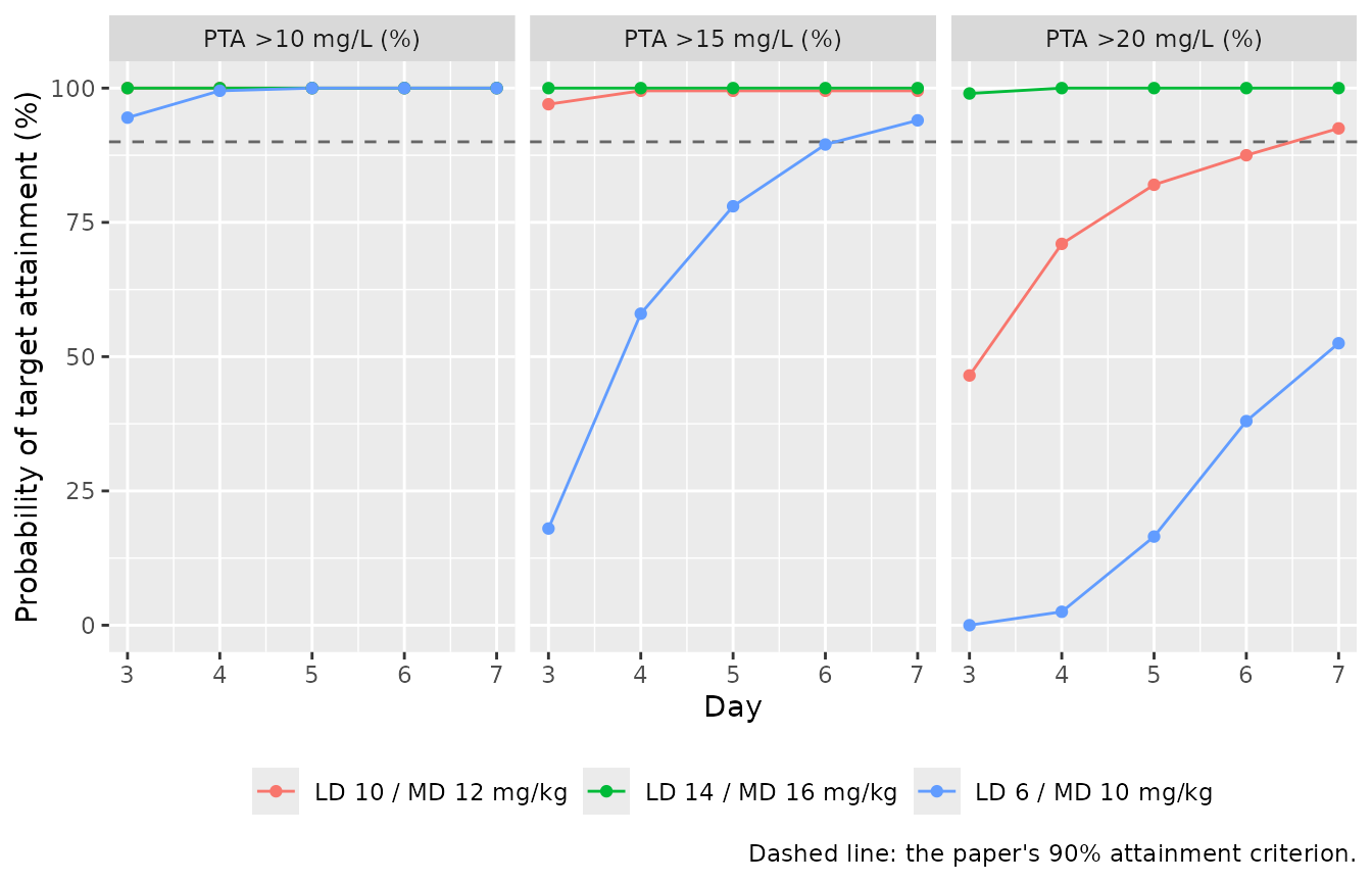
Probability of target attainment for trough targets of 10, 15 and 20 mg/L on days 3-7. Replicates Figure 2 of Kim 2024 (q24h maintenance arm).
cell <- function(reg, day, col) {
  v <- pta[[col]][pta$regimen == reg & pta$Day == day]
  if (length(v) != 1L) stop("no unique row for '", reg, "' on day ", day)
  v
}
days <- 3:7

claims <- tibble::tribble(
  ~Claim, ~Achieved, ~Gate,
  "LD 6 / MD 10 mg/kg q24h: Ctrough >10 mg/L in >=90%, days 3-7 (Section 3.4, Figure 2)",
    min(vapply(days, cell, numeric(1), reg = "LD 6 / MD 10 mg/kg", col = "PTA >10 mg/L (%)")), TRUE,
  "LD 14 / MD 16 mg/kg q24h: Ctrough >20 mg/L in >=90%, days 3-7 (Section 3.4, Figure 2)",
    min(vapply(days, cell, numeric(1), reg = "LD 14 / MD 16 mg/kg", col = "PTA >20 mg/L (%)")), TRUE,
  "LD 10 / MD 12 mg/kg q24h: Ctrough >15 mg/L in >90%, days 4-7 (Section 4)",
    min(vapply(4:7, cell, numeric(1), reg = "LD 10 / MD 12 mg/kg", col = "PTA >15 mg/L (%)")), TRUE,
  "LD 10 / MD 12 mg/kg q24h: Ctrough >15 mg/L in >90% on day 3 (Section 4)",
    cell("LD 10 / MD 12 mg/kg", 3, "PTA >15 mg/L (%)"), FALSE,
  "LD 10 / MD 12 mg/kg q24h does NOT reach 90% for Ctrough >20 mg/L on day 3 ('LDs and MDs had to be over 14 mg/kg', Section 3.4)",
    cell("LD 10 / MD 12 mg/kg", 3, "PTA >20 mg/L (%)"), TRUE
)
claims$Pass <- c(
  claims$Achieved[1] >= 90,
  claims$Achieved[2] >= 90,
  claims$Achieved[3] >= 90,
  claims$Achieved[4] >= 90,
  claims$Achieved[5] <  90
)

knitr::kable(claims, digits = 1,
caption = "Published dosing claims vs. the packaged model. `Gate = FALSE` rows are reported but not asserted (see below).")| Claim | Achieved | Gate | Pass |
|---|---|---|---|
| LD 6 / MD 10 mg/kg q24h: Ctrough >10 mg/L in >=90%, days 3-7 (Section 3.4, Figure 2) | 97.5 | TRUE | TRUE |
| LD 14 / MD 16 mg/kg q24h: Ctrough >20 mg/L in >=90%, days 3-7 (Section 3.4, Figure 2) | 97.5 | TRUE | TRUE |
| LD 10 / MD 12 mg/kg q24h: Ctrough >15 mg/L in >90%, days 4-7 (Section 4) | 98.5 | TRUE | TRUE |
| LD 10 / MD 12 mg/kg q24h: Ctrough >15 mg/L in >90% on day 3 (Section 4) | 95.0 | FALSE | TRUE |
| LD 10 / MD 12 mg/kg q24h does NOT reach 90% for Ctrough >20 mg/L on day 3 (‘LDs and MDs had to be over 14 mg/kg’, Section 3.4) | 48.0 | TRUE | TRUE |
# Nephrotoxicity marker: the paper reports the proportion with Ctrough > 60 mg/L
# as "0 ... and only a few exhibited values less than 1%" for q24h maintenance
# (Section 3.4). Asserted as a mean below the paper's own 1% bound rather than as
# an exact zero, which would be a single-draw assertion.
stopifnot(mean(pta$`Ctrough >60 mg/L (%)`) < 1)

# Gated claims only. Row 4 is excluded: its realised value sits roughly 1.5
# Monte-Carlo standard errors above the 90% threshold at 200 subjects per arm
# (MC-SE ~1.8 percentage points at p = 0.93), so gating it would be close to a
# coin flip on a CI runner drawing a different cohort. It is reported instead.
stopifnot(all(claims$Pass[claims$Gate]))
Assumptions and deviations
- Sampling-window midpoints. Kim 2024 sampled once in a 48-120 h window and once in a 168-240 h window without reporting the realised times per subject. The NCA above places those two samples at 84 h (the midpoint of the stated window) and 192 h (the median Tlast reported in Table 3). All other sampling times are exact. The choice was made before any comparison was run; PKNCA’s automatic terminal-slope window then selects 3 or 4 points per subject, which is what Kim 2024 Section 3.3 reports.
- Covariate distributions. Body weight and BSA-adjusted CKD-EPI creatinine eGFR are drawn independently from log-normal distributions matched to the mean and CV% in Kim 2024 Table 1 (weight 64.8 kg, CV 19.9%; eGFR 103 mL/min, CV 15.5%). The paper does not report the joint distribution or the weight-eGFR correlation, and the two are positively correlated in reality because the eGFR is de-normalized by body surface area. Simulating them independently slightly widens the spread of clearance per kilogram relative to the real cohort. Sex, age, height and body surface area are not model covariates and are not simulated.
- Monte Carlo virtual patients. Kim 2024’s dosing simulations used 5000 virtual patients whose covariate distribution the paper does not describe. The reproduction here uses 200 subjects per regimen (the nlmixr2lib cohort cap) drawn from the distributions above, so the attainment percentages carry a Monte-Carlo standard error of roughly 1-2 percentage points and will not match the paper’s to the decimal.
- The day-3 Ctrough > 15 mg/L claim is reported, not gated. It reproduces (93% against the paper’s “>90%”), but the margin is within about 1.5 Monte-Carlo standard errors of the threshold at 200 subjects per arm. Asserting it would produce a check that flips between machines rather than one that detects a transcription error. The three claims with real headroom are gated.
-
IIV percentage convention. Kim 2024 Table 2 labels
each IIV simply as a percentage without stating whether it is
sqrt(omega^2)orsqrt(exp(omega^2) - 1). The log-normal conventionomega^2 = log(1 + CV^2)is used, matching the rest of nlmixr2lib. The two conventions differ by at most 3% relative on the largest IIV in this model (32.7% on Q2) and by well under 1% on the four fixed IIVs, so the choice is not material to any result above. -
Fixed IIVs. The BSV on CL, V1, V2 and V3 was fixed
by the authors because the corresponding RSEs exceeded 25% (Kim 2024
Section 3.2 and Section 4). Those four etas carry
fixed()inini(); Q2 and Q3 do not. No variance was invented - every value comes from Table 2. -
Covariate units. The
CRCLcolumn in this model holds the CKD-EPI creatinine eGFR de-normalized to the individual’s body surface area, in raw mL/min - not mL/min/1.73 m^2. The 105.27 mL/min reference in Table 2 is on that scale. Supplying a BSA-normalized value would misstate the covariate; seecovariateData$CRCL$notesin the model file. - Single-dose data, multiple-dose simulation. The model was fitted to a single 200 mg dose. The dosing simulations above extrapolate to repeated 6-16 mg/kg doses, exactly as Kim 2024 did; the paper defends this on the grounds that the simulated range sits inside teicoplanin’s stated 2-25 mg/kg linear range (Section 4, limitation 3).
- No errata. No corrigendum or author correction to this article was found on the MDPI article page or in PubMed at the time of extraction.