Cabozantinib exposure-response in renal cell carcinoma (Lacy 2018)
Source:vignettes/articles/Lacy_2018_cabozantinib_exposure_response.Rmd
Lacy_2018_cabozantinib_exposure_response.RmdModel and source
Lacy 2018 develops three independent exposure-response analyses in adults with advanced renal cell carcinoma (RCC) enrolled in the phase III METEOR study (cabozantinib 60 mg tablet QD with allowed reduction to 40 mg / 20 mg vs everolimus 10 mg QD; PFS, ORR, and OS endpoints):
- A longitudinal sum-of-tumor-diameter (SOD) growth-inhibition PD model with first-order growth, an attenuating saturable cabozantinib drug effect, and acquired resistance.
- A repeated time-to-event (RTTE) hazard model for “dose modification of any kind” (DMAK) with a two-state on-dose vs dose-hold hazard.
- Cox proportional-hazards (PH) survival models in SAS PROC PHREG for progression-free survival (PFS) and six safety endpoints, each reported as covariate beta coefficients on top of a non-parametric empirical baseline hazard.
The first two are parametric pharmacometric models and are extracted as separate model files in nlmixr2lib:
-
modellib("Lacy_2018_cabozantinib_tumor")– tumor growth model. -
modellib("Lacy_2018_cabozantinib_dose_modification")– DMAK hazard model.
The Cox PH models (PFS and safety endpoints) are not extracted as
standalone model files. PROC PHREG provides covariate beta coefficients
only; the baseline hazard h0(t) is non-parametric
(empirical KM-style) and is not reported in the paper, so the Cox models
cannot be simulated forward in rxode2 without an external assumption
about the baseline form. The beta coefficients themselves are tabulated
below for reference.
The upstream popPK model that produces the drug input Cavg (carried
as the time-varying CAV covariate column) is
modellib("Lacy_2018_cabozantinib"), extracted from the
companion Lacy 2018 popPK manuscript (doi:10.1007/s00280-018-3581-0). Lacy 2018 ER does not
redevelop the popPK; it uses individual empirical-Bayes post-hoc
parameters from the companion paper to derive Cavg per subject and
time.
- Citation: Lacy S, Nielsen J, Yang B, Miles D, Nguyen L, Hutmacher M. Population exposure-response analysis of cabozantinib efficacy and safety endpoints in patients with renal cell carcinoma. Cancer Chemother Pharmacol. 2018;81(6):1061-1070. doi:10.1007/s00280-018-3579-7. Upstream popPK (driver of CAV): Lacy S et al., Cancer Chemother Pharmacol. 2018;81(6):1071-1082; doi:10.1007/s00280-018-3581-0; see modellib(‘Lacy_2018_cabozantinib’).
- Article: https://doi.org/10.1007/s00280-018-3579-7
- Companion popPK: https://doi.org/10.1007/s00280-018-3581-0
Population
METEOR randomised 658 adults with advanced or metastatic clear-cell RCC who had received at least one prior VEGFR-TKI therapy to cabozantinib (n = 330) or everolimus (n = 328). The Lacy 2018 ER analyses use the cabozantinib arm:
- PFS Cox PH model: n = 315 (paper Supplemental Table 1).
- DMAK RTTE model: n = 317 with 0-52 events per patient.
- Tumor growth model: n = 319 with 1637 evaluable tumor diameter measurements.
Baseline cohort characteristics are in Lacy 2018 ER Supplemental Table 2: ECOG score (50% 0, 46% 1, 2% 2, 3% missing), MSKCC risk factors (46% / 42% / 13% favorable / intermediate / poor), baseline SOD relative to the cohort median (50% below, 50% above), visceral and bone metastases (18% yes), lung metastases (62% yes), liver metastases (27% yes), bone metastases (23% yes), prior number of VEGF-target TKI therapies (71% one, 29% two-or-more), number of organs involved (most patients had two or more), and time to progressive disease for most recent prior TKI (13% under 3 months, 86% at-or-over 3 months).
The same information is available programmatically:
readModelDb("Lacy_2018_cabozantinib_tumor")$population
readModelDb("Lacy_2018_cabozantinib_dose_modification")$population
Source trace
Per-parameter provenance is recorded as in-file comments on each
ini() entry in
inst/modeldb/specificDrugs/Lacy_2018_cabozantinib_tumor.R
and
inst/modeldb/specificDrugs/Lacy_2018_cabozantinib_dose_modification.R.
The table collects the trail in one place.
| Equation / parameter | Value | Source location |
|---|---|---|
Tumor growth equation
dY/dt = k_grow*Y - decay(t)*Y*Cavg/(EC50+Cavg)
|
n/a | Eq. 5, paper Methods “Longitudinal sum of tumor diameter model” |
Tumor
decay(t) = k_dmax + k_dmax_tot * exp(-k_tol * t)
|
n/a | Paper Methods Eq. 5 narrative; attenuation half-life 25.6 days in Results |
lrbase_tumor -> baseline SOD |
63.1 mm | ER Supplemental Table 3 (longitudinal tumor growth row) |
lkgrow |
0.00155 1/day | ER Supplemental Table 3 |
lkdmax |
0.00125 1/day | ER Supplemental Table 3 |
lkdmaxtot |
0.00835 1/day | ER Supplemental Table 3 |
lktol |
0.0271 1/day | ER Supplemental Table 3 (half-life log(2)/k_tol = 25.6 d in Results) |
lec50 |
251 ng/mL | ER Supplemental Table 3 (paper Results: EC80 ~ 1000 ng/mL confirms) |
Tumor addSd
|
5.75 mm | ER Supplemental Table 3 (“Residual Variability (SD) (mm)”) |
| Tumor IIVs | see model file | ER Supplemental Table 3 |
| DMAK hazard equation | n/a | Eqs. 6-8, paper Methods “Dose modification” subsection |
lhaz_base -> theta_base |
-5.4 | ER Supplemental Table 3 (all dose modification RTTE row) |
e_cav_haz -> theta_drug |
0.000807 per ng/mL | ER Supplemental Table 3 |
lhaz_base_hold -> theta_base-hold |
-2.7 | ER Supplemental Table 3 |
| DMAK IIV on lhaz_base | 0.655 (variance) | ER Supplemental Table 3 |
Virtual cohort
The original observed data are not publicly available. The figures below use a simple three-cohort design that holds the daily cabozantinib dose constant at 20, 40, and 60 mg and uses the paper’s reported steady-state average concentrations as the time-invariant CAV input (375, 750, 1125 ng/mL respectively, ER Results). This isolates the structural exposure-response behaviour from the additional dynamics of the DMAK dose-modification process; the paper’s full Figure-5 simulation co-integrates DMAK and tumor growth and is discussed under Assumptions and deviations below.
set.seed(2018L)

# Three constant-dose, constant-CAV cohorts at the METEOR starting doses.
cohorts <- tibble::tribble(
  ~cohort, ~daily_dose_mg, ~cavg_ng_ml,
  "20 mg",  20,            375,
  "40 mg",  40,            750,
  "60 mg",  60,           1125
)

# Daily observation grid over a 365-day simulation horizon.
obs_times <- seq(0, 365, by = 7)

make_subject_rows <- function(id, dose_mg, cavg) {
  tibble::tibble(
    id   = id,
    time = obs_times,
    evid = 0L,
    DOSE = dose_mg,
    CAV  = cavg
  )
}

n_per_cohort <- 100L

events <- dplyr::bind_rows(lapply(seq_len(nrow(cohorts)), function(k) {
  id_offset <- (k - 1L) * n_per_cohort
  dplyr::bind_rows(lapply(seq_len(n_per_cohort), function(j) {
    make_subject_rows(id     = id_offset + j,
                      dose_mg = cohorts$daily_dose_mg[k],
                      cavg    = cohorts$cavg_ng_ml[k])
  })) |>
    dplyr::mutate(cohort = cohorts$cohort[k])
})) |>
  dplyr::arrange(id, time)

stopifnot(!anyDuplicated(unique(events[, c("id", "time")])))
Tumor growth simulation
mod_tumor <- readModelDb("Lacy_2018_cabozantinib_tumor")
sim_tumor <- rxode2::rxSolve(mod_tumor, events = events,
                             keep = c("cohort", "DOSE", "CAV"))
#> ℹ parameter labels from comments will be replaced by 'label()'
sim_tumor <- as.data.frame(sim_tumor)
Figure 5 – median percent change in tumor diameter
Replicates the qualitative shape of Figure 5 of Lacy 2018 ER (median percent change in target-lesion SOD over 1 year by starting dose). Because this vignette holds CAV constant per cohort (no dose modifications), the simulated medians are deeper than the paper’s DMAK-coupled simulation (paper: -4.5% / -9.1% / -11.9% for 20 / 40 / 60 mg starting dose; this vignette: see plot caption).
tum_summary <- sim_tumor |>
  dplyr::group_by(cohort, time) |>
  dplyr::summarise(
    median_change_pct = stats::median((tumor_size / 63.1 - 1) * 100,
                                      na.rm = TRUE),
    .groups = "drop"
  )

ggplot(tum_summary, aes(time, median_change_pct, colour = cohort)) +
  geom_line(linewidth = 1) +
  geom_hline(yintercept = 0, linetype = "dashed", colour = "grey50") +
  scale_x_continuous(breaks = c(0, 60, 120, 180, 240, 300, 365)) +
  labs(x = "Time (days)",
       y = "Median percent change from baseline (%)",
       colour = "Starting dose",
       title = "Figure 5 -- median tumor SOD change at constant CAV",
       caption = "Constant-CAV virtual cohort; paper Figure 5 uses DMAK-coupled dynamic CAV.")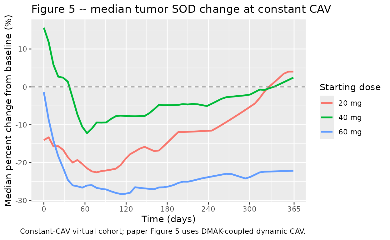
Replicates Figure 5 of Lacy 2018 ER (median percent change from baseline tumor SOD at 20, 40, 60 mg starting doses, virtual cohort with constant CAV).
end_tumor <- sim_tumor |>
  dplyr::filter(time == max(obs_times)) |>
  dplyr::group_by(cohort) |>
  dplyr::summarise(
    median_change_pct = round(stats::median((tumor_size / 63.1 - 1) * 100,
                                            na.rm = TRUE), 1),
    .groups = "drop"
  ) |>
  dplyr::left_join(
    tibble::tibble(
      cohort                  = c("20 mg", "40 mg", "60 mg"),
      paper_change_pct        = c(-4.5, -9.1, -11.9)
    ),
    by = "cohort"
  )

knitr::kable(end_tumor,
             caption = paste0("End-of-year median percent change from baseline ",
"(this vignette vs Lacy 2018 ER Results / Table 1)."))| cohort | median_change_pct | paper_change_pct |
|---|---|---|
| 20 mg | 4.0 | -4.5 |
| 40 mg | 2.4 | -9.1 |
| 60 mg | -22.2 | -11.9 |
The simulated medians at constant CAV are systematically lower (more tumor shrinkage) than the paper’s reported medians because the paper’s simulation lets the DMAK process reduce or interrupt the dose over the year, lowering the time-averaged exposure relative to the per-cohort steady-state CAV used here. See Assumptions and deviations.
EC50 sensitivity at EC80 ~ 1000 ng/mL
Paper Results: “The EC50 is 251 ng/mL and the EC80 value is about 1000 ng/mL”. A quick sanity check confirms the saturable drug effect plateaus near the 60-mg starting-dose Cavg:
cavg_grid <- c(0, 100, 251, 500, 750, 1000, 1125, 2000)
ec50      <- 251
tibble::tibble(
  cavg_ng_ml      = cavg_grid,
  drug_fraction   = round(cavg_grid / (ec50 + cavg_grid), 3)
) |>
knitr::kable(caption = "Saturable Cavg / (EC50 + Cavg) at EC50 = 251 ng/mL.")| cavg_ng_ml | drug_fraction |
|---|---|
| 0 | 0.000 |
| 100 | 0.285 |
| 251 | 0.500 |
| 500 | 0.666 |
| 750 | 0.749 |
| 1000 | 0.799 |
| 1125 | 0.818 |
| 2000 | 0.888 |
The Cavg = 1000 row should give 1000 / 1251 = 0.799 (~ EC80), matching the paper’s stated value.
Dose-modification (DMAK) simulation
The DMAK model is a repeated TTE hazard model with two states (active
dose, dose hold). For an at-rest typical subject the per-day
instantaneous hazard during active dose is
exp(theta_base + theta_drug * CAV) and during a dose hold
is exp(theta_base_hold); eta on the active baseline
contributes the subject-level random effect.
mod_dmak <- readModelDb("Lacy_2018_cabozantinib_dose_modification")

dmak_events <- events |> dplyr::select(id, time, evid, DOSE, CAV, cohort)

sim_dmak <- rxode2::rxSolve(mod_dmak, events = dmak_events,
                            keep = c("cohort", "DOSE", "CAV"))
#> ℹ parameter labels from comments will be replaced by 'label()'
sim_dmak <- as.data.frame(sim_dmak)
dmak_summary <- sim_dmak |>
  dplyr::group_by(cohort, time) |>
  dplyr::summarise(
    sur_median = stats::median(sur, na.rm = TRUE),
    .groups = "drop"
  )

ggplot(dmak_summary, aes(time, sur_median, colour = cohort)) +
  geom_line(linewidth = 1) +
  scale_x_continuous(breaks = c(0, 60, 120, 180, 240, 300, 365)) +
  scale_y_continuous(limits = c(0, 1)) +
  labs(x = "Time (days)",
       y = "Median dose-modification-free survival",
       colour = "Starting dose",
       title = "DMAK hazard model -- median survival by cohort",
       caption = "Constant CAV per cohort; no dose hold. Survival = exp(-cumhaz).")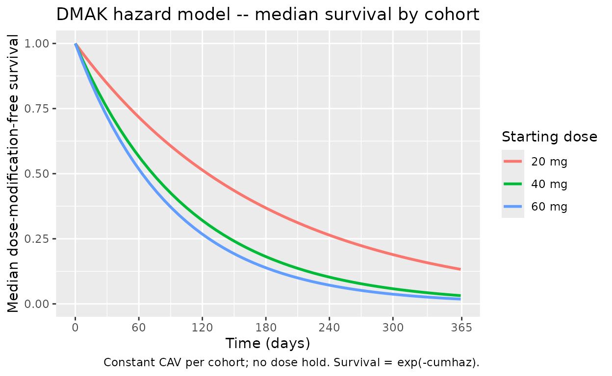
Predicted dose-modification-free survival probability over 1 year for 20, 40, 60 mg constant-dose cohorts (no dose hold). The 60 mg cohort accumulates DMAK events faster, reflecting the higher CAV and the +0.000807 per ng/mL effect on the log hazard.
# Reproduce a per-day hazard ratio of 60 mg vs 20 mg from the typical
# active-dose hazard expression. The mu in the model file is theta_drug =
# e_cav_haz = 0.000807 per ng/mL of CAV, so HR(60 mg vs 20 mg) =
# exp(theta_drug * (CAV_60 - CAV_20)).
theta_drug <- 0.000807
cav_60     <- 1125
cav_20     <- 375
hr_60_20   <- exp(theta_drug * (cav_60 - cav_20))
tibble::tibble(
  comparison              = c("60 mg vs 40 mg", "60 mg vs 20 mg"),
  delta_cav_ng_ml         = c(cav_60 - 750, cav_60 - cav_20),
  hazard_ratio            = c(exp(theta_drug * (cav_60 - 750)), hr_60_20)
) |>
  knitr::kable(digits = 3,
caption = "Active-dose DMAK hazard ratio derived from theta_drug.")| comparison | delta_cav_ng_ml | hazard_ratio |
|---|---|---|
| 60 mg vs 40 mg | 375 | 1.353 |
| 60 mg vs 20 mg | 750 | 1.832 |
Cox PH endpoint summary (not extracted as standalone models)
Lacy 2018 ER reports Cox PH analyses for progression-free survival
and six adverse-event endpoints in SAS PROC PHREG. These provide
covariate beta coefficients only; the baseline hazard h0(t)
is non-parametric (empirical, computed by PHREG against the METEOR
dataset) and is not itself reported in the paper, so the models cannot
be simulated forward in rxode2 without an external baseline-hazard
assumption. The beta coefficients are listed here for reference.
cox_ph <- tibble::tribble(
  ~endpoint,                          ~term,                                     ~estimate,    ~standard_error,
  "Progression-free survival",        "beta_TR-CAVG3W",                          -1.25581,     0.63139,
  "Progression-free survival",        "beta_ECOG_score_ge1",                      0.85058,     0.50374,
  "Progression-free survival",        "beta_TR-CAVG3W_x_ECOG_ge1",               -0.31399,     0.61166,
  "Progression-free survival",        "beta_SOD_gt_median",                       0.84555,     0.49149,
  "Progression-free survival",        "beta_TR-CAVG3W_x_SOD_gt_median",          -1.25269,     0.59989,
  "Progression-free survival",        "beta_liver_mets_yes",                      1.32190,     0.50495,
  "Progression-free survival",        "beta_TR-CAVG3W_x_liver_mets",             -1.26391,     0.62994,
  "Progression-free survival",        "beta_MET_IHC_high",                        1.18288,     0.59877,
  "Progression-free survival",        "beta_TR-CAVG3W_x_MET_IHC_high",           -1.63127,     0.76851,
  "Progression-free survival",        "beta_TR-CAVG3W_x_prior_TKI_PD_lt_3mo",     0.81809,     0.24775,
  "Fatigue / asthenia (grade >= 3)",  "beta_CAVG2W",                              0.0009319,   0.000338,
  "Palmar-plantar erythrodysesthesia","beta_CAVG2W",                              0.00106,     0.0002208,
  "Nausea / vomiting (grade >= 3)",   "beta_CAVG2W",                              0.00104,     0.0005360,
  "Diarrhea (grade >= 3)",            "beta_CAVG2W",                              0.0007653,   0.0003351,
  "Stomatitis (grade >= 3)",          "beta_CAVG0T",                              0.00169,     0.0008533,
  "Hypertension (SBP > 160 or DBP > 100)", "beta_CAVGID",                         0.0008187,   0.0002234
)

knitr::kable(cox_ph, digits = 7,
caption = "Lacy 2018 ER Supplemental Table 4 Cox PH beta coefficients.")| endpoint | term | estimate | standard_error |
|---|---|---|---|
| Progression-free survival | beta_TR-CAVG3W | -1.2558100 | 0.6313900 |
| Progression-free survival | beta_ECOG_score_ge1 | 0.8505800 | 0.5037400 |
| Progression-free survival | beta_TR-CAVG3W_x_ECOG_ge1 | -0.3139900 | 0.6116600 |
| Progression-free survival | beta_SOD_gt_median | 0.8455500 | 0.4914900 |
| Progression-free survival | beta_TR-CAVG3W_x_SOD_gt_median | -1.2526900 | 0.5998900 |
| Progression-free survival | beta_liver_mets_yes | 1.3219000 | 0.5049500 |
| Progression-free survival | beta_TR-CAVG3W_x_liver_mets | -1.2639100 | 0.6299400 |
| Progression-free survival | beta_MET_IHC_high | 1.1828800 | 0.5987700 |
| Progression-free survival | beta_TR-CAVG3W_x_MET_IHC_high | -1.6312700 | 0.7685100 |
| Progression-free survival | beta_TR-CAVG3W_x_prior_TKI_PD_lt_3mo | 0.8180900 | 0.2477500 |
| Fatigue / asthenia (grade >= 3) | beta_CAVG2W | 0.0009319 | 0.0003380 |
| Palmar-plantar erythrodysesthesia | beta_CAVG2W | 0.0010600 | 0.0002208 |
| Nausea / vomiting (grade >= 3) | beta_CAVG2W | 0.0010400 | 0.0005360 |
| Diarrhea (grade >= 3) | beta_CAVG2W | 0.0007653 | 0.0003351 |
| Stomatitis (grade >= 3) | beta_CAVG0T | 0.0016900 | 0.0008533 |
| Hypertension (SBP > 160 or DBP > 100) | beta_CAVGID | 0.0008187 | 0.0002234 |
The PFS Cox PH uses a transformed nonlinear cabozantinib effect
TR-CAVG3W = -Cavg3w / (EC50 + Cavg3w) with EC50 = 100 ng/mL
fixed (paper Methods “Progression-free survival”); the per-AE Cox PH
models use a linear cabozantinib effect on the indicated exposure window
(CAVG2W = 2-week rolling mean; CAVG1D = 24-h rolling mean; CAVG0T =
average from time 0 to event). Predicted hazard ratios at the predicted
60-mg steady-state Cavg relative to the 20-mg Cavg are reported as 2.21
(PPES), 2.01 (fatigue / asthenia), 1.85 (hypertension), and 1.78
(diarrhea) (paper Abstract).
Assumptions and deviations
-
Cavg as constant per cohort. The paper’s Figure 5
simulation co-integrates the DMAK process and the tumor growth model:
the DMAK fires events that change DOSE, dynamic CAV is recomputed from
the new dose via the upstream popPK, and the tumor growth ODE consumes
that dynamic CAV. Reproducing that full pipeline requires a custom
event-resolver loop outside
rxSolve. This vignette holds CAV constant at the per-cohort steady-state value (375 / 750 / 1125 ng/mL) so the tumor and DMAK structural behaviour can be inspected independently. The expected consequence is that the simulated end-of-year tumor change is systematically deeper than the paper’s DMAK-coupled prediction. -
Upstream popPK fixed to typical-value posthoc. When
a user wants to drive CAV from
Lacy_2018_cabozantinib(the companion popPK), they should run the popPK first to generate empirical-Bayes individual Cavg = AUC_tau / tau per subject and per dose interval, then carry CAV as a time-varying column into the tumor and DMAK models. The popPK vignetteLacy_2018_cabozantinib.Rmdwalks the cohort construction; this vignette skips that step for brevity. -
DMAK IIV attached to active-state baseline only.
The paper reports a single “IIV baseline” of 0.655 in ER Supplemental
Table 3 and does not state which state’s baseline the eta attaches to.
This extraction applies the eta only to the active-dose log hazard
(
lhaz_base), matching the paper’s “baseline” symbol convention. An alternative interpretation – a subject-level eta shared between the active and dose-hold states – is mathematically defensible and would couple a patient’s dose-modification proneness across both states. -
IIV reported as variance under the “(omega)” label.
Lacy 2018 ER Supplemental Table 3 reports IIVs under the column header
“(omega)” with a typical-value-like back-transformation. The values
(e.g. 0.522 for baseline tumor IIV) reproduce the paper’s reported CV =
72% via the linearised approximation
sqrt(omega^2) ~ CV, indicating that the reported values are omega^2 (variance) rather than omega (SD). This extraction uses the values directly as variance, matching the convention used by the companion popPK model (Lacy 2018 popPK Table 3 footnote d, which reports omega^2 explicitly). -
Supplement labels “k_dmax_tot” in the structural row and
“k_dmax_tol” in the IIV row. Treated here as a supplement typo
for the same parameter (
k_dmax_tot); the IIV is wired to the attenuating-decay-rate magnitude. -
Cox PH PFS and AE models not extracted. The Cox PH
models in this paper are SAS PROC PHREG fits with non-parametric
empirical baseline hazards. The paper does not report
h0(t)in a form that can be simulated forward in rxode2 (e.g. a Weibull / Gompertz parameterisation), so the Cox PH models cannot be encoded as standalone simulation models without operator-chosen fabricated baselines. The beta coefficients are tabulated above for reference; a future “Cox PH parametric-baseline” extension could encode them as parametric hazard models if and when an operator decides which baseline form to assume.