Model and source
- Citation: Liu W, Tan Z, Yang P, Yu Z, Yao X, Zhou P, Liu L, Zhou W. Model-based exploration of the rationality of off-label use of cetirizine in Chinese pediatric patients: a prospective cohort study. Front Pharmacol. 2024;15:1322788. doi:10.3389/fphar.2024.1322788. Final parameter estimates are Supplementary Table S1. The covariate equations are not printed in Liu 2024 and are taken from the base model it re-fitted: Pitsiu M, Hussein Z, Majid O, Aarons L, de Longueville M, Stockis A. Retrospective population pharmacokinetic analysis of cetirizine in children aged 6 months to 12 years. Br J Clin Pharmacol. 2004;57(4):402-411. doi:10.1046/j.1365-2125.2003.02017.x (Table 4).
- Description: One-compartment population PK model with first-order absorption and first-order elimination for oral cetirizine in Chinese children (about 0.5-12 years) with allergic diseases (Liu 2024). The structure is the Pitsiu 2004 paediatric cetirizine model re-fitted to sparse real-world Chinese data: CL/F is linear in age with sex-specific intercepts (CL/F = 0.28 * AGE + 0.771 [male] or 0.592 [female] L/h), V/F is linear in age (V/F = 23.1 + 1.42 * AGE L), and ka = theta_ka + CL/V guards against flip-flop. The age slope on CL/F, the V/F intercept, the IIV on CL/F and V/F and the proportional residual error were re-estimated; the sex intercepts, the V/F age slope, theta_ka and its IIV were held fixed at the Pitsiu 2004 values.
- Article: https://doi.org/10.3389/fphar.2024.1322788 (open access; the parameter table is Supplementary Table S1)
- Structural source: Pitsiu et al. 2004, https://doi.org/10.1046/j.1365-2125.2003.02017.x (free full text in PubMed Central, PMC1884474)
Liu 2024 did not build a new structural model. Its sparse real-world
data (up to three samples per child, few in the absorption phase) were
used to re-fit the Pitsiu 2004 paediatric cetirizine model. After an
external evaluation showed misspecification across the exposure range,
the age slope on CL/F, the V/F intercept, the IIV on CL/F and V/F and
the proportional residual error were re-estimated. All absorption
parameters, both sex-specific CL/F intercepts and the V/F age slope
stayed fixed at the Pitsiu 2004 values. Liu 2024 describes the covariate
relationships in prose only. The equations below are the ones printed in
Pitsiu 2004 Table 4, and the parameter names in Liu’s Supplementary
Table S1 (CL_AGE, CL_SEX on Male,
CL_SEX on Female, V, V_AGE,
Ka) map onto them one to one:
- CL/F (L/h) =
CL_AGEx AGE +CL_SEX,Mx (1 - SEXF) +CL_SEX,Fx SEXF - V/F (L) =
V+V_AGEx AGE - ka (1/h) = theta_ka + CL/V
Population
Liu 2024 ran a prospective cohort study at Peking University Third Hospital (April 2020 to April 2021) in 63 Chinese children with allergic diseases (38 male, 25 female). They were aged 6.34 +/- 3.7 years, weighed 26.4 +/- 15.7 kg and were 120.1 +/- 27.7 cm tall (Results 3.1). Thirty-nine children received label doses and 24 received off-label doses of up to twice the label dose (Table 1); five of those exceeded 0.25 mg/kg per administration (Table 3). Children with abnormal liver or kidney function were excluded. Each child gave up to three plasma samples, measured by HPLC-MS/MS.
The same information is available programmatically:
str(readModelDb("Liu_2024_cetirizine")()$population)
#> List of 15
#>  $ species       : chr "human"
#>  $ n_subjects    : int 63
#>  $ n_studies     : int 1
#>  $ age_range     : chr "Under 14 years at enrolment; Table 1 age groups 0.5-2, 2-6 and 6-12 years"
#>  $ age_mean      : chr "6.34 +/- 3.7 years"
#>  $ weight_mean   : chr "26.4 +/- 15.7 kg"
#>  $ height_mean   : chr "120.1 +/- 27.7 cm"
#>  $ sex_female_pct: num 39.7
#>  $ race_ethnicity: chr "Chinese (100%)"
#>  $ disease_state : chr "Children with allergic diseases (allergic rhinitis, urticaria, asthma and others) prescribed oral cetirizine; n"| __truncated__
#>  $ dose_range    : chr "Label doses 2.5 mg bid (0.5-6 years) or 5 mg bid (6-12 years); 24 of 63 children received off-label doses up to"| __truncated__
#>  $ regions       : chr "China (Peking University Third Hospital, Beijing)"
#>  $ samples       : chr "Up to three plasma samples per child; 85 concentrations in the NPDE evaluation (Supplementary Figure S4). Plasm"| __truncated__
#>  $ estimation    : chr "NONMEM 7.4.4, FOCE-I"
#>  $ notes         : chr "Prospective cohort study, April 2020 - April 2021: 38 male and 25 female children, 39 at label doses and 24 at "| __truncated__
Source trace
| Equation / parameter | Value | Source location |
|---|---|---|
lcl (CL/F intercept, male) |
fixed(log(0.771)) L/h |
Liu 2024 Table S1 ‘CL_SEX on Male’ 0.771 FIXED; Pitsiu 2004 Table 4 |
lcl_female (CL/F intercept, female) |
fixed(log(0.592)) L/h |
Liu 2024 Table S1 ‘CL_SEX on Female’ 0.592 FIXED; Pitsiu 2004 Table 4 |
e_age_cl |
0.28 L/h/year | Liu 2024 Table S1 ‘CL_AGE’ (RSE 17%); Discussion 4.1 ‘0.28 in our results’ |
lvc (V/F intercept) |
log(23.1) L |
Liu 2024 Table S1 ‘V’ (RSE 40%) |
e_age_vc |
fixed(1.42) L/year |
Liu 2024 Table S1 ‘V_AGE’ 1.42 FIXED; Pitsiu 2004 Table 4 |
lka (theta_ka) |
fixed(log(2.14)) 1/h |
Liu 2024 Table S1 ‘Ka’ 2.14 FIXED; Pitsiu 2004 Table 4 |
etalcl |
0.378 | Liu 2024 Table S1 ‘IIV_CL/F’ (RSE 34%, shrinkage 21.2%) |
etalvc |
0.445 | Liu 2024 Table S1 ‘IIV_V/F’ (RSE 41%, shrinkage 47.1%) |
etalka |
fixed(2.1) |
Liu 2024 Table S1 ‘IIV_Ka’ 2.1 FIXED (Pitsiu 2004: 145% CV, 1.45^2 = 2.10) |
propSd |
0.36 | Liu 2024 Table S1 ‘Proportional error’ (RSE 16%); ‘Sigma’ 1 FIXED |
| CL/F, V/F equations | n/a | Pitsiu 2004 Table 4; Liu 2024 Methods 2.4.2 (prose) |
| ka = theta_ka + CL/V | n/a | Pitsiu 2004 Table 4 footnote; Liu 2024 Methods 2.4.2 |
| One compartment, first-order absorption | n/a | Liu 2024 Methods 2.4.2 |
Cc = central / vc * 1000 (ng/mL) |
n/a | Unit conversion: dose in mg, V/F in L |
Typical CL/F and V/F by age: Liu 2024 vs Pitsiu 2004
Re-estimating the age slope on CL/F (0.12 to 0.28 L/h/year) and the V/F intercept (4.00 to 23.1 L) gives Chinese children a higher clearance and a much larger apparent volume than the Pitsiu 2004 European children of the same age. The table sets the typical values of both models against each other, with the Pitsiu values from Pitsiu 2004 Table 5.
mod <- readModelDb("Liu_2024_cetirizine")
th <- rxode2::rxode(mod)$theta
#> ℹ parameter labels from comments will be replaced by 'label()'
ages <- c(0.5, 2, 6, 7, 12)
typical <- tibble(AGE = ages) |>
  mutate(
    liu_cl_m = th[["e_age_cl"]] * AGE + exp(th[["lcl"]]),
    liu_cl_f = th[["e_age_cl"]] * AGE + exp(th[["lcl_female"]]),
    liu_v = exp(th[["lvc"]]) + th[["e_age_vc"]] * AGE,
    pitsiu_cl_m = c(0.83, 1.01, 1.49, 1.61, 2.21),
    pitsiu_cl_f = c(0.65, 0.83, 1.31, 1.43, 2.03),
    pitsiu_v = c(4.71, 6.84, 12.5, 13.9, 21.0)
  )
typical |>
  dplyr::rename(
    "Age (years)" = AGE,
    "Liu CL/F male (L/h)" = liu_cl_m,
    "Liu CL/F female (L/h)" = liu_cl_f,
    "Liu V/F (L)" = liu_v,
    "Pitsiu CL/F male (L/h)" = pitsiu_cl_m,
    "Pitsiu CL/F female (L/h)" = pitsiu_cl_f,
    "Pitsiu V/F (L)" = pitsiu_v
  ) |>
knitr::kable(digits = 2, caption = "Typical apparent clearance and volume by age.")| Age (years) | Liu CL/F male (L/h) | Liu CL/F female (L/h) | Liu V/F (L) | Pitsiu CL/F male (L/h) | Pitsiu CL/F female (L/h) | Pitsiu V/F (L) |
|---|---|---|---|---|---|---|
| 0.5 | 0.91 | 0.73 | 23.81 | 0.83 | 0.65 | 4.71 |
| 2.0 | 1.33 | 1.15 | 25.94 | 1.01 | 0.83 | 6.84 |
| 6.0 | 2.45 | 2.27 | 31.62 | 1.49 | 1.31 | 12.50 |
| 7.0 | 2.73 | 2.55 | 33.04 | 1.61 | 1.43 | 13.90 |
| 12.0 | 4.13 | 3.95 | 40.14 | 2.21 | 2.03 | 21.00 |
The model reproduces Pitsiu’s Table 5 exactly when Pitsiu’s own estimates (0.12 L/h/year and 4.00 L) replace Liu’s. That confirms the equations encoded here are the ones Pitsiu printed:
pitsiu_check <- typical |>
  mutate(
    cl_m = 0.12 * AGE + exp(th[["lcl"]]),
    cl_f = 0.12 * AGE + exp(th[["lcl_female"]]),
    v = 4.00 + th[["e_age_vc"]] * AGE
  )
# Pitsiu Table 5 is printed to 2-3 significant figures.
stopifnot(
  max(abs(pitsiu_check$cl_m - pitsiu_check$pitsiu_cl_m)) < 0.011,
  max(abs(pitsiu_check$cl_f - pitsiu_check$pitsiu_cl_f)) < 0.011,
  max(abs(pitsiu_check$v - pitsiu_check$pitsiu_v)) < 0.06
)
Virtual cohort: the twelve label-dose patients of Table 2
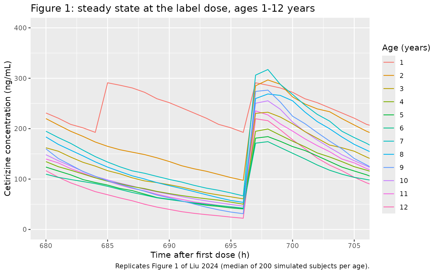
Liu 2024 Table 2 lists twelve virtual girls aged 1 to 12 years, each at the maximum label dose, and reports the median steady-state Cmax and Cmin over 1,000 simulations. Body weight and height are listed in that table but are not model covariates. Each patient is simulated here with 200 subjects (the package’s per-arm cap), dosed for 30 days. The last 24 hours, 696 to 720 h, are the steady-state window; Figure 1 of the paper covers the same window.
table2 <- tibble::tribble(
  ~pid, ~regimen, ~amt, ~ii, ~AGE, ~SEXF, ~cmax_pub, ~cmin_pub,
  1, "2.5 mg bid", 2.5, 12, 1, 1, 232.27, 156.48,
  2, "5 mg qd", 5, 24, 2, 1, 243.06, 86.27,
  3, "5 mg qd", 5, 24, 3, 1, 225.75, 71.94,
  4, "5 mg qd", 5, 24, 4, 1, 204.98, 47.53,
  5, "5 mg qd", 5, 24, 5, 1, 186.70, 48.09,
  6, "5 mg qd", 5, 24, 6, 1, 160.15, 31.70,
  7, "10 mg qd", 10, 24, 7, 1, 306.93, 55.57,
  8, "10 mg qd", 10, 24, 8, 1, 270.42, 38.28,
  9, "10 mg qd", 10, 24, 9, 1, 259.97, 32.19,
  10, "10 mg qd", 10, 24, 10, 1, 227.78, 37.98,
  11, "10 mg qd", 10, 24, 11, 1, 234.20, 28.80,
  12, "10 mg qd", 10, 24, 12, 1, 209.28, 18.94
) |>
  mutate(patient = sprintf("Age %d y, %s", AGE, regimen))

n_per_patient <- 200
t_end <- 720
t_ss <- t_end - 24

make_patient <- function(row, id_offset) {
  ids <- id_offset + seq_len(n_per_patient)
  dose_times <- seq(0, t_end - row$ii, by = row$ii)
  obs_times <- seq(t_ss - 16, t_end, by = 0.25)
  doses <- tidyr::expand_grid(id = ids, time = dose_times) |>
    mutate(amt = row$amt, evid = 1L, cmt = "depot")
  obs <- tidyr::expand_grid(id = ids, time = obs_times) |>
    mutate(amt = 0, evid = 0L, cmt = "central")
  bind_rows(doses, obs) |>
    mutate(AGE = row$AGE, SEXF = row$SEXF, patient = row$patient)
}

events <- bind_rows(lapply(seq_len(nrow(table2)), function(i) {
  make_patient(table2[i, ], id_offset = (i - 1L) * n_per_patient)
})) |>
  arrange(id, time, desc(evid))
stopifnot(!anyDuplicated(unique(events[, c("id", "time", "evid")])))
Simulation
rxode2::rxSetSeed(20240314)
sim <- rxode2::rxSolve(mod, events = events, keep = c("patient")) |>
  as.data.frame()
#> ℹ parameter labels from comments will be replaced by 'label()'
Replicate Figure 1
Figure 1 of Liu 2024 plots one curve per age over the steady-state window. The paper does not say whether that curve is the typical value or the median of the simulations. The median curve is plotted here, on the paper’s hourly grid.
median_curve <- sim |>
  filter(abs(time - round(time)) < 1e-9) |>
  group_by(patient, time) |>
  summarise(Cc = median(Cc), .groups = "drop") |>
  left_join(table2 |> select(patient, AGE), by = "patient")

ggplot(median_curve, aes(time, Cc, colour = factor(AGE), group = patient)) +
  geom_line() +
  coord_cartesian(xlim = c(680, 705), ylim = c(0, 400)) +
  labs(
    x = "Time after first dose (h)", y = "Cetirizine concentration (ng/mL)",
    colour = "Age (years)",
    title = "Figure 1: steady state at the label dose, ages 1-12 years",
    caption = "Replicates Figure 1 of Liu 2024 (median of 200 simulated subjects per age)."
  )
PKNCA validation against Table 2
PKNCA computes Cmax and Cmin per subject over the steady-state window. The median across the 200 subjects of each patient is compared with Table 2.
sim_nca <- sim |>
  dplyr::filter(!is.na(Cc), time >= t_ss) |>
  dplyr::select(id, time, Cc, patient)

dose_df <- events |>
  dplyr::filter(evid == 1, time >= t_ss) |>
  dplyr::select(id, time, amt, patient)

conc_obj <- PKNCA::PKNCAconc(sim_nca, Cc ~ time | patient + id)
dose_obj <- PKNCA::PKNCAdose(dose_df, amt ~ time | patient + id)
intervals <- data.frame(start = t_ss, end = t_end, cmax = TRUE, cmin = TRUE, tmax = TRUE)
nca_res <- PKNCA::pk.nca(PKNCA::PKNCAdata(conc_obj, dose_obj, intervals = intervals))

published <- table2 |>
  select(patient, cmax = cmax_pub, cmin = cmin_pub)

cmp <- nlmixr2lib::ncaComparisonTable(
  simulated = nca_res,
  reference = published,
  by = "patient",
  units = c(cmax = "ng/mL", cmin = "ng/mL"),
  tolerance_pct = 20
)
knitr::kable(
  cmp,
  caption = "Median simulated vs. published (Table 2) steady-state Cmax and Cmin. * differs from reference by >20%."
)| NCA parameter | patient | Reference | Simulated | % diff |
|---|---|---|---|---|
| Cmax (ng/mL) | Age 1 y, 2.5 mg bid | 232 | 297 | +28.0%* |
| Cmax (ng/mL) | Age 2 y, 5 mg qd | 243 | 310 | +27.7%* |
| Cmax (ng/mL) | Age 3 y, 5 mg qd | 226 | 250 | +10.9% |
| Cmax (ng/mL) | Age 4 y, 5 mg qd | 205 | 216 | +5.2% |
| Cmax (ng/mL) | Age 5 y, 5 mg qd | 187 | 204 | +9.0% |
| Cmax (ng/mL) | Age 6 y, 5 mg qd | 160 | 188 | +17.6% |
| Cmax (ng/mL) | Age 7 y, 10 mg qd | 307 | 347 | +12.9% |
| Cmax (ng/mL) | Age 8 y, 10 mg qd | 270 | 292 | +7.9% |
| Cmax (ng/mL) | Age 9 y, 10 mg qd | 260 | 307 | +17.9% |
| Cmax (ng/mL) | Age 10 y, 10 mg qd | 228 | 281 | +23.5%* |
| Cmax (ng/mL) | Age 11 y, 10 mg qd | 234 | 259 | +10.6% |
| Cmax (ng/mL) | Age 12 y, 10 mg qd | 209 | 246 | +17.5% |
| Cmin (ng/mL) | Age 1 y, 2.5 mg bid | 156 | 193 | +23.1%* |
| Cmin (ng/mL) | Age 2 y, 5 mg qd | 86.3 | 97.6 | +13.1% |
| Cmin (ng/mL) | Age 3 y, 5 mg qd | 71.9 | 60.8 | -15.6% |
| Cmin (ng/mL) | Age 4 y, 5 mg qd | 47.5 | 50.2 | +5.6% |
| Cmin (ng/mL) | Age 5 y, 5 mg qd | 48.1 | 40.8 | -15.2% |
| Cmin (ng/mL) | Age 6 y, 5 mg qd | 31.7 | 42.3 | +33.4%* |
| Cmin (ng/mL) | Age 7 y, 10 mg qd | 55.6 | 66.6 | +19.9% |
| Cmin (ng/mL) | Age 8 y, 10 mg qd | 38.3 | 53.7 | +40.3%* |
| Cmin (ng/mL) | Age 9 y, 10 mg qd | 32.2 | 31.3 | -2.8% |
| Cmin (ng/mL) | Age 10 y, 10 mg qd | 38 | 46.3 | +21.9%* |
| Cmin (ng/mL) | Age 11 y, 10 mg qd | 28.8 | 41.1 | +42.9%* |
| Cmin (ng/mL) | Age 12 y, 10 mg qd | 18.9 | 22.2 | +17.4% |
The simulated troughs scatter on both sides of Table 2. Most are within about 25%; the misses run both high and low, which looks like Monte-Carlo noise in a 200-subject median of a highly variable trough rather than a bias. The per-subject median Cmax is consistently above Table 2, by roughly 5-30%. That is what you would expect if the paper read Cmax off the median concentration-time curve on an hourly grid (the curve of its Figure 1), not as the median of per-subject maxima: with an absorption rate constant as variable as this one (fixed IIV variance 2.1), subjects peak at different times, so the median of the individual peaks sits above the peak of the median curve. The same metric taken from the median curve agrees more closely:
curve_metric <- median_curve |>
  filter(time >= t_ss) |>
  group_by(patient) |>
  summarise(cmax_sim = max(Cc), cmin_sim = min(Cc), .groups = "drop") |>
  left_join(table2 |> select(pid, patient, cmax_pub, cmin_pub), by = "patient") |>
  arrange(pid) |>
  mutate(
    cmax_pct = 100 * (cmax_sim / cmax_pub - 1),
    cmin_pct = 100 * (cmin_sim / cmin_pub - 1)
  )

curve_metric |>
  select(patient, cmax_sim, cmax_pub, cmax_pct, cmin_sim, cmin_pub, cmin_pct) |>
  dplyr::rename(
    "Patient" = patient,
    "Cmax,ss sim (ng/mL)" = cmax_sim,
    "Cmax,ss Table 2" = cmax_pub,
    "Cmax diff (%)" = cmax_pct,
    "Cmin,ss sim (ng/mL)" = cmin_sim,
    "Cmin,ss Table 2" = cmin_pub,
    "Cmin diff (%)" = cmin_pct
  ) |>
knitr::kable(digits = 1, caption = "Peak and trough of the median curve (hourly grid) vs. Table 2.")| Patient | Cmax,ss sim (ng/mL) | Cmax,ss Table 2 | Cmax diff (%) | Cmin,ss sim (ng/mL) | Cmin,ss Table 2 | Cmin diff (%) |
|---|---|---|---|---|---|---|
| Age 1 y, 2.5 mg bid | 291.0 | 232.3 | 25.3 | 192.6 | 156.5 | 23.1 |
| Age 2 y, 5 mg qd | 296.7 | 243.1 | 22.1 | 97.6 | 86.3 | 13.1 |
| Age 3 y, 5 mg qd | 232.6 | 225.8 | 3.0 | 60.8 | 71.9 | -15.6 |
| Age 4 y, 5 mg qd | 199.3 | 205.0 | -2.8 | 50.2 | 47.5 | 5.6 |
| Age 5 y, 5 mg qd | 184.2 | 186.7 | -1.3 | 40.8 | 48.1 | -15.2 |
| Age 6 y, 5 mg qd | 174.2 | 160.2 | 8.8 | 42.3 | 31.7 | 33.4 |
| Age 7 y, 10 mg qd | 317.3 | 306.9 | 3.4 | 66.6 | 55.6 | 19.9 |
| Age 8 y, 10 mg qd | 268.8 | 270.4 | -0.6 | 53.7 | 38.3 | 40.3 |
| Age 9 y, 10 mg qd | 276.4 | 260.0 | 6.3 | 31.3 | 32.2 | -2.8 |
| Age 10 y, 10 mg qd | 255.3 | 227.8 | 12.1 | 46.3 | 38.0 | 21.9 |
| Age 11 y, 10 mg qd | 235.3 | 234.2 | 0.5 | 41.1 | 28.8 | 42.9 |
| Age 12 y, 10 mg qd | 219.6 | 209.3 | 4.9 | 22.2 | 18.9 | 17.4 |
# Structural check on the centre of the twelve patients. A mis-transcribed
# clearance slope (0.12 vs 0.28 L/h/year) or volume intercept (4.0 vs 23.1 L)
# moves these medians by far more than 25%; the per-patient values carry the
# Monte-Carlo noise of 200 subjects and the unknown details of the paper's
# summary, so no per-patient bound is asserted. Across draws the medians
# were about +4% to +9% (Cmax) and +8% to +19% (Cmin); the trough of a
# 200-subject cohort is the noisier of the two, hence its wider bound.
stopifnot(
  abs(median(curve_metric$cmax_pct)) < 20,
  abs(median(curve_metric$cmin_pct)) < 35
)
For ages 3 to 12 the median-curve peak is within about 15% of Table 2. The youngest patients (1 year on 2.5 mg bid and 2 years on 5 mg qd) come out about 10-25% higher than Table 2; the source does not report enough about its simulation to explain the difference.
The paper’s main finding is reproduced by the typical-value (no IIV) curves. Among the label doses the 7-year-old has the highest steady-state peak (the first age at 10 mg qd) and the 6-year-old the lowest (the oldest age at 5 mg qd), because the label dose steps up with age while CL/F and V/F rise continuously:
sim_tv <- rxode2::rxSolve(
  rxode2::zeroRe(mod),
  events = events |> filter(id %% n_per_patient == 1),
  keep = c("patient")
) |>
  as.data.frame()
#> ℹ parameter labels from comments will be replaced by 'label()'
#> ℹ omega/sigma items treated as zero: 'etalcl', 'etalvc', 'etalka'
#> Warning: multi-subject simulation without without 'omega'

tv_peaks <- sim_tv |>
  filter(time >= t_ss) |>
  group_by(patient) |>
  summarise(cmax_typical = max(Cc), .groups = "drop") |>
  left_join(table2 |> select(pid, patient, AGE), by = "patient") |>
  arrange(pid)
knitr::kable(
  tv_peaks |> select(patient, cmax_typical) |>
    dplyr::rename("Patient" = patient, "Typical Cmax,ss (ng/mL)" = cmax_typical),
  digits = 1
)| Patient | Typical Cmax,ss (ng/mL) |
|---|---|
| Age 1 y, 2.5 mg bid | 278.9 |
| Age 2 y, 5 mg qd | 273.4 |
| Age 3 y, 5 mg qd | 235.0 |
| Age 4 y, 5 mg qd | 208.3 |
| Age 5 y, 5 mg qd | 188.3 |
| Age 6 y, 5 mg qd | 172.6 |
| Age 7 y, 10 mg qd | 319.9 |
| Age 8 y, 10 mg qd | 298.7 |
| Age 9 y, 10 mg qd | 280.6 |
| Age 10 y, 10 mg qd | 265.0 |
| Age 11 y, 10 mg qd | 251.3 |
| Age 12 y, 10 mg qd | 239.1 |
Off-label and overdose scenarios
Table 3 patients (doses above 0.25 mg/kg)
Liu 2024 Table 3 reports Bayesian (POSTHOC) simulations of five children who received more than 0.25 mg/kg per dose. Those values use each child’s individual random effects, which are not published. The population-level prediction for the same age, sex and regimen is shown for context only and is not expected to match.
table3 <- tibble::tribble(
  ~patient_id, ~amt, ~AGE, ~SEXF, ~cmax_pub, ~cmin_pub,
  "6", 6.43, 4.08, 0, 417.67, 237.31,
  "45", 5, 6, 1, 236.64, 100.48,
  "54", 5, 5.7, 0, 266.31, 135.87,
  "58", 5, 5, 0, 277.34, 150.08,
  "66", 9, 4, 0, 580.68, 325.40
)

ev_t3 <- bind_rows(lapply(seq_len(nrow(table3)), function(i) {
  r <- table3[i, ]
  ids <- (i - 1L) * n_per_patient + seq_len(n_per_patient)
  bind_rows(
    tidyr::expand_grid(id = ids, time = seq(0, 216 - 12, by = 12)) |>
      mutate(amt = r$amt, evid = 1L, cmt = "depot"),
    tidyr::expand_grid(id = ids, time = seq(192, 216, by = 1)) |>
      mutate(amt = 0, evid = 0L, cmt = "central")
  ) |>
    mutate(AGE = r$AGE, SEXF = r$SEXF, patient_id = r$patient_id)
})) |>
  arrange(id, time, desc(evid))

sim_t3 <- rxode2::rxSolve(mod, events = ev_t3, keep = c("patient_id")) |>
  as.data.frame()

sim_t3 |>
  filter(time >= 204) |>
  group_by(patient_id, time) |>
  summarise(Cc = median(Cc), .groups = "drop") |>
  group_by(patient_id) |>
  summarise(cmax_sim = max(Cc), cmin_sim = min(Cc), .groups = "drop") |>
  left_join(table3, by = "patient_id") |>
  arrange(as.integer(patient_id)) |>
  select(patient_id, amt, AGE, cmax_sim, cmax_pub, cmin_sim, cmin_pub) |>
  dplyr::rename(
    "Patient" = patient_id,
    "Dose bid (mg)" = amt,
    "Age (years)" = AGE,
    "Cmax,ss population (ng/mL)" = cmax_sim,
    "Cmax,ss Table 3 POSTHOC" = cmax_pub,
    "Cmin,ss population (ng/mL)" = cmin_sim,
    "Cmin,ss Table 3 POSTHOC" = cmin_pub
  ) |>
knitr::kable(digits = 1, caption = "Population predictions for the Table 3 regimens (context only).")| Patient | Dose bid (mg) | Age (years) | Cmax,ss population (ng/mL) | Cmax,ss Table 3 POSTHOC | Cmin,ss population (ng/mL) | Cmin,ss Table 3 POSTHOC |
|---|---|---|---|---|---|---|
| 6 | 6.4 | 4.1 | 379.9 | 417.7 | 199.5 | 237.3 |
| 45 | 5.0 | 6.0 | 246.5 | 236.6 | 123.1 | 100.5 |
| 54 | 5.0 | 5.7 | 242.0 | 266.3 | 116.4 | 135.9 |
| 58 | 5.0 | 5.0 | 258.4 | 277.3 | 109.0 | 150.1 |
| 66 | 9.0 | 4.0 | 554.6 | 580.7 | 258.4 | 325.4 |
Figure 3: the 30 mg medication error
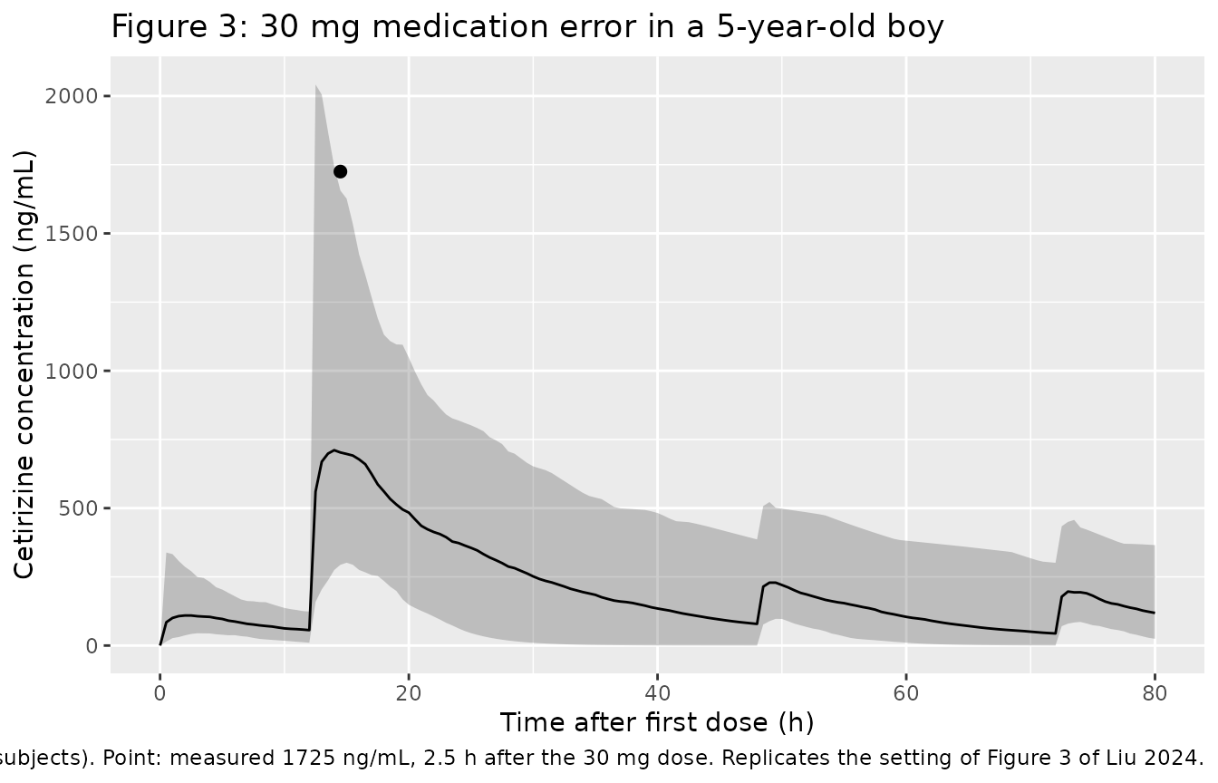
A 5-year-old boy prescribed 5 mg bid was given a single 30 mg dose 12 h after his first 5 mg dose. A sample taken 2.5 h after the error measured 1725 ng/mL. Dosing restarted later. The curve in Figure 3 of the paper doses again at about 48 and 72 h, which is the schedule simulated here. Figure 3 is the boy’s individual POSTHOC curve, which needs his unpublished random effects. The population prediction interval below is shown with the measured concentration for orientation.
ids_od <- seq_len(n_per_patient)
ev_od <- bind_rows(
  tidyr::expand_grid(id = ids_od, tibble(time = c(0, 12, 48, 72), amt = c(5, 30, 5, 5))) |>
    mutate(evid = 1L, cmt = "depot"),
  tidyr::expand_grid(id = ids_od, time = seq(0, 80, by = 0.5)) |>
    mutate(amt = 0, evid = 0L, cmt = "central")
) |>
  mutate(AGE = 5, SEXF = 0) |>
  arrange(id, time, desc(evid))

sim_od <- rxode2::rxSolve(mod, events = ev_od) |> as.data.frame()

od_summary <- sim_od |>
  group_by(time) |>
  summarise(
    Q05 = quantile(Cc, 0.05), Q50 = median(Cc), Q95 = quantile(Cc, 0.95),
    .groups = "drop"
  )

ggplot(od_summary, aes(time, Q50)) +
  geom_ribbon(aes(ymin = Q05, ymax = Q95), alpha = 0.25) +
  geom_line() +
  geom_point(data = data.frame(time = 14.5, Q50 = 1725), colour = "black", size = 2) +
  labs(
    x = "Time after first dose (h)", y = "Cetirizine concentration (ng/mL)",
    title = "Figure 3: 30 mg medication error in a 5-year-old boy",
    caption = paste(
      "Population median and 90% interval (200 subjects). Point: measured",
      "1725 ng/mL, 2.5 h after the 30 mg dose. Replicates the setting of Figure 3 of Liu 2024."
    )
  )
od_summary |>
  filter(time == 14.5) |>
  dplyr::rename(
    "Time (h)" = time, "5th percentile" = Q05, "Median" = Q50, "95th percentile" = Q95
  ) |>
knitr::kable(digits = 1, caption = "Population prediction 2.5 h after the 30 mg dose (ng/mL).")| Time (h) | 5th percentile | Median | 95th percentile |
|---|---|---|---|
| 14.5 | 293.9 | 702.7 | 1655.8 |
The measured 1725 ng/mL lies well above the population median, in the upper tail of the interval. The paper’s individual fit, which uses the boy’s own random effects, passes a peak of about 1,780 ng/mL through it.
Assumptions and deviations
-
Equations from Pitsiu 2004. Liu 2024 names the
covariate effects (
CL_AGE,CL_SEX,V,V_AGE) but does not print the equations. They were taken from Pitsiu 2004 Table 4, the model Liu re-fitted. The Pitsiu typical-value check above reproduces Pitsiu’s Table 5 from those equations. - Concentration units. Liu 2024 Tables 2 and 3 and the Results text label concentrations as ug/mL, but the axes of Figures 1-3 read ng/mL, Pitsiu 2004 modelled ng/mL from doses in ug, and 10 mg into a V/F of about 30 L can only give hundreds of ng/mL. The model reports ng/mL, and the ug/mL labels in the paper are treated as a typographical error.
- IIV values are variances. Liu’s Table S1 IIV column is read as the NONMEM OMEGA variance. The fixed ka entry, 2.1, is exactly the square of the 145% CV Pitsiu reported (1.45^2 = 2.10), which identifies the scale.
- Residual error. Table S1 lists a ‘Proportional error’ of 0.36 alongside ‘Sigma 1 FIXED’. This is the THETA-scaled residual form, so 0.36 is the proportional SD.
- No bioavailability term. CL/F and V/F are apparent parameters and the oral dose enters the depot with F = 1, as in Pitsiu 2004.
-
Sex coding. Pitsiu coded SEX = 1 for female, which
is the canonical
SEXFdirectly. - Cohort size. Table 2 summarises 1,000 simulations per patient. This vignette uses 200 per patient, so the per-patient medians carry more Monte-Carlo noise than the paper’s.
- Steady-state window. The paper does not state how long it dosed before reading steady state. Figure 1’s axis (680-705 h) and the doses at 684 and 696 h suggest about 30 days, which is what is simulated here.
- Cohort size reported inconsistently. The modelling text gives 63 children, but Table 1 adds up to 65 across age groups and the safety section refers to 66 patients. The population metadata uses 63.
- No correction notice for Liu 2024 or Pitsiu 2004 was found in Europe PMC as of 2026-10-29.