Actinomycin-D (Mondick 2006)
Source:vignettes/articles/Mondick_2006_dactinomycin.Rmd
Mondick_2006_dactinomycin.RmdModel and source
- Citation: Mondick JT, Gibiansky L, Gastonguay MR, Veal GJ, Barrett JS. Acknowledging Parameter Uncertainty in the Simulation-Based Design of an Actinomycin-D Pharmacokinetic Study in Pediatric Patients with Wilms’ Tumor or Rhabdomyosarcoma. PAGE 15 (2006) Abstr 938. https://www.page-meeting.org/?abstract=938
- Description: Three-compartment intravenous population PK model for actinomycin-D (dactinomycin) in 33 pediatric and young-adult patients (1.58-20.3 years) with Wilms’ tumor or rhabdomyosarcoma. All disposition parameters are allometrically scaled by total body weight, normalized to a reference weight of 70 kg, with theory-based fixed exponents (0.75 on clearances, 1.0 on volumes; not explicitly stated in the abstract). Inter-individual variability was reported only for V1 (54.4% CV) and CL (57.2% CV); residual error and the remaining IIV terms (V2, V3, Q2, Q3) were not reported in the source conference abstract and are encoded as fixed(0). Mondick 2006 (PAGE 15 Abstr 938).
- Article: PAGE 15 (2006) Abstr 938
Population
Mondick 2006 (PAGE 15 Abstr 938) constructed a population PK model for actinomycin-D (AMD; dactinomycin) from 33 pediatric and young-adult patients (age 1.58-20.3 years) with Wilms’ tumor or rhabdomyosarcoma receiving AMD as part of their standard chemotherapy regimen. Age, gender, and body size were screened as candidate covariates; only body-weight allometric scaling (normalized to a reference weight of 70 kg) was retained in the final model. The abstract does not print the cohort body-weight distribution or sex breakdown. Infants under 12 months were not represented in the developmental cohort, and the abstract’s principal motivation is to design a prospective Children’s Oncology Group Phase I Consortium trial to fill that gap. The trial design proposed in the abstract calls for 200 patients randomized to one of two sparse-sampling schemes:
- Scheme 1: 5 min, 10 min, 2-3 h, 24-28 h, and 48-96 h post-dose
- Scheme 2: 5 min, 0.75-1.5 h, 5-6 h, 24-28 h, and 48-96 h post-dose
A sample-size analysis in the same abstract concluded that 50 subjects under one year of age would be required to detect a 30 percent change in clearance in that subpopulation.
The same information is available programmatically via
readModelDb("Mondick_2006_dactinomycin")$population.
Source trace
Per-parameter origin is recorded as an in-file comment next to each
ini() entry in
inst/modeldb/specificDrugs/Mondick_2006_dactinomycin.R. The
table below collects them for review.
| Equation / parameter | Value | Source location |
|---|---|---|
| Structural model | three-compartment IV with body-weight allometric scaling | Mondick 2006 Results: “AMD pharmacokinetics were well described by a three-compartment model with all parameters allometrically scaled by total body weight, normalized to a weight of 70 kg.” |
lvc (V1 at WT = 70 kg) |
log(3.88) L |
Mondick 2006 Results: V1 = 3.88 L (CV 54.4 percent) |
lvp (V2 at WT = 70 kg) |
log(443) L |
Mondick 2006 Results: V2 = 443 L |
lvp2 (V3 at WT = 70 kg) |
log(23.7) L |
Mondick 2006 Results: V3 = 23.7 L |
lcl (CL at WT = 70 kg) |
log(8.27) L/h |
Mondick 2006 Results: CL = 8.27 L/h (CV 57.2 percent) |
lq (Q2 at WT = 70 kg) |
log(252) L/h |
Mondick 2006 Results: Q2 = 252 L/h |
lq2 (Q3 at WT = 70 kg) |
log(12.7) L/h |
Mondick 2006 Results: Q3 = 12.7 L/h |
etalvc IIV |
log(1 + 0.544^2) = 0.259 |
Mondick 2006 Results: V1 %CV = 54.4 |
etalcl IIV |
log(1 + 0.572^2) = 0.283 |
Mondick 2006 Results: CL %CV = 57.2 |
etalvp, etalvp2, etalq,
etalq2
|
fixed(0) |
Not reported in Mondick 2006 abstract; encoded as fixed per nlmixr2lib policy for unreported IIV with structural values present. |
e_wt_cl (allometric exp on CL/Q) |
fixed(0.75) |
Not printed in abstract; theory-based Holford/Anderson exponent assumed (see Assumptions and deviations). |
e_wt_vc (allometric exp on V) |
fixed(1.0) |
Not printed in abstract; theory-based Holford/Anderson exponent assumed (see Assumptions and deviations). |
propSd |
fixed(0) |
Not reported in Mondick 2006 abstract; encoded as fixed per nlmixr2lib policy for unreported RUV with structural values present. Simulations from this packaging are deterministic typical-value trajectories on the propSd axis. |
Virtual cohort
The Mondick 2006 abstract does not publish per-subject demographics or a body-weight distribution. The virtual cohort below spans the study’s stated age range (1.58-20.3 years) plus an extrapolation panel for infants under one year (the prospective-trial subpopulation the paper is designed to estimate). Approximate weight-for-age uses mid-range pediatric estimates; the simulations are sensitive only to body weight via the allometric scaling, not to age per se.
set.seed(20060938L)  # PAGE 15 Abstr 938

# Four age strata x 50 subjects each = 200 subjects total (within the
# 200/arm vignette cap). Each cohort has a disjoint ID range so a
# bind_rows() does not collide on the ID key inside rxSolve.
make_stratum <- function(n, age_lo, age_hi, wt_lo, wt_hi, label, id_offset) {
  tibble::tibble(
    id        = id_offset + seq_len(n),
    AGE       = runif(n, min = age_lo, max = age_hi),
    WT        = runif(n, min = wt_lo,  max = wt_hi),
    ageGroup  = label
  )
}

cohort <- dplyr::bind_rows(
  make_stratum(50, 0.25,  1.00,  5,  10, "Infant (<1 yr, extrapolation)", id_offset =   0L),
  make_stratum(50, 1.58,  6.00, 12,  22, "Toddler / young child (1.58-6 yr)", id_offset =  50L),
  make_stratum(50, 6.00, 12.00, 22,  45, "Older child (6-12 yr)",        id_offset = 100L),
  make_stratum(50, 12.0, 20.30, 45,  70, "Adolescent / young adult (12-20.3 yr)", id_offset = 150L)
)

knitr::kable(
  cohort |>
    group_by(ageGroup) |>
    summarise(
      n          = dplyr::n(),
      AGE_range  = sprintf("%.2f-%.2f", min(AGE), max(AGE)),
      WT_range   = sprintf("%.1f-%.1f", min(WT),  max(WT)),
      .groups    = "drop"
    ),
  caption = "Virtual cohort summary: 200 subjects across four age strata. Body weight is the only model covariate."
)| ageGroup | n | AGE_range | WT_range |
|---|---|---|---|
| Adolescent / young adult (12-20.3 yr) | 50 | 12.01-20.17 | 45.1-69.7 |
| Infant (<1 yr, extrapolation) | 50 | 0.26-0.98 | 5.0-10.0 |
| Older child (6-12 yr) | 50 | 6.03-11.97 | 22.8-44.2 |
| Toddler / young child (1.58-6 yr) | 50 | 1.61-5.95 | 12.0-21.7 |
Simulation
Each subject receives a single 1.25 mg/m^2 IV bolus dose of actinomycin-D (the typical pediatric AMD dose), capped at 2 mg, with body surface area approximated from the body-weight Mosteller-style relation BSA ~ sqrt(WT / 36). Observation times reproduce the union of the two proposed sampling schemes from the abstract.
# Per-subject events: 1 IV bolus into central + observation grid that
# spans both abstract-defined sparse sampling schemes.
obs_grid <- c(
  0.0833,                # 5 min
  0.1667,                # 10 min
  seq(0.75, 1.5, by = 0.25),  # 0.75-1.5 h (scheme 2)
  2, 3,                  # 2-3 h (scheme 1)
  5, 6,                  # 5-6 h (scheme 2)
  24, 26, 28,            # 24-28 h
  48, 72, 96             # 48-96 h
) |>
  sort() |>
  unique()

# Add a dense grid for plotting smooth Cc(t) curves on top of the
# sparse-sample times.
plot_grid <- sort(unique(c(obs_grid, seq(0, 96, by = 0.5))))

per_subject_events <- function(subj) {
  bsa  <- sqrt(subj$WT / 36)               # m^2 (Mosteller approximation)
  amt  <- pmin(1.25 * bsa, 2)              # mg (1.25 mg/m^2 capped at 2 mg)

  dose <- tibble::tibble(
    id   = subj$id, time = 0, amt = amt, cmt = "central", evid = 1L
  )
  obs  <- tibble::tibble(
    id   = subj$id, time = plot_grid, amt = 0, cmt = NA_character_, evid = 0L
  )
  dplyr::bind_rows(dose, obs) |>
    dplyr::mutate(WT = subj$WT, AGE = subj$AGE, ageGroup = subj$ageGroup) |>
    dplyr::arrange(time, dplyr::desc(evid))
}

events <- dplyr::bind_rows(
  lapply(seq_len(nrow(cohort)), function(i) per_subject_events(cohort[i, ]))
)
stopifnot(!anyDuplicated(unique(events[, c("id", "time", "evid")])))
mod <- rxode2::rxode2(readModelDb("Mondick_2006_dactinomycin"))
#> ℹ parameter labels from comments will be replaced by 'label()'
sim <- rxode2::rxSolve(mod, events = events, keep = c("WT", "AGE", "ageGroup"))
#> ℹ omega/sigma items treated as zero: 'etalvp', 'etalvp2', 'etalq', 'etalq2'
The packaged model encodes residual error as fixed(0)
because the Mondick 2006 abstract does not report a residual error
model; the simulation above is therefore a stochastic VPC over the two
reported IIVs (etalvc, etalcl) only.
Replicate published figures
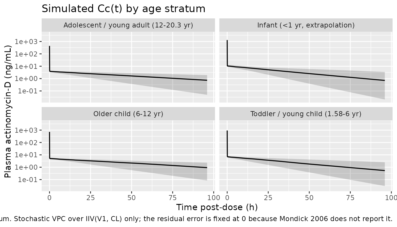
The abstract does not include a published concentration-time figure, but it does propose two sparse-sampling designs to be used in the prospective trial. The panel below shows simulated typical-value Cc(t) for each age stratum on a semi-log y-axis, with the two proposed sampling schemes overlaid as vertical guides.
sim |>
  dplyr::filter(!is.na(Cc), Cc > 0) |>
  dplyr::group_by(time, ageGroup) |>
  dplyr::summarise(
    Q05 = stats::quantile(Cc, 0.05, na.rm = TRUE),
    Q50 = stats::quantile(Cc, 0.50, na.rm = TRUE),
    Q95 = stats::quantile(Cc, 0.95, na.rm = TRUE),
    .groups = "drop"
  ) |>
  ggplot(aes(time, Q50)) +
  geom_ribbon(aes(ymin = Q05, ymax = Q95), alpha = 0.2) +
  geom_line(linewidth = 0.6) +
  facet_wrap(~ageGroup) +
  scale_y_log10() +
  labs(
    x       = "Time post-dose (h)",
    y       = "Plasma actinomycin-D (ng/mL)",
    title   = "Simulated Cc(t) by age stratum",
    caption = "Median (line) and 5-95 percentile envelope (band) across 50 subjects per stratum. Stochastic VPC over IIV(V1, CL) only; the residual error is fixed at 0 because Mondick 2006 does not report it."
  )
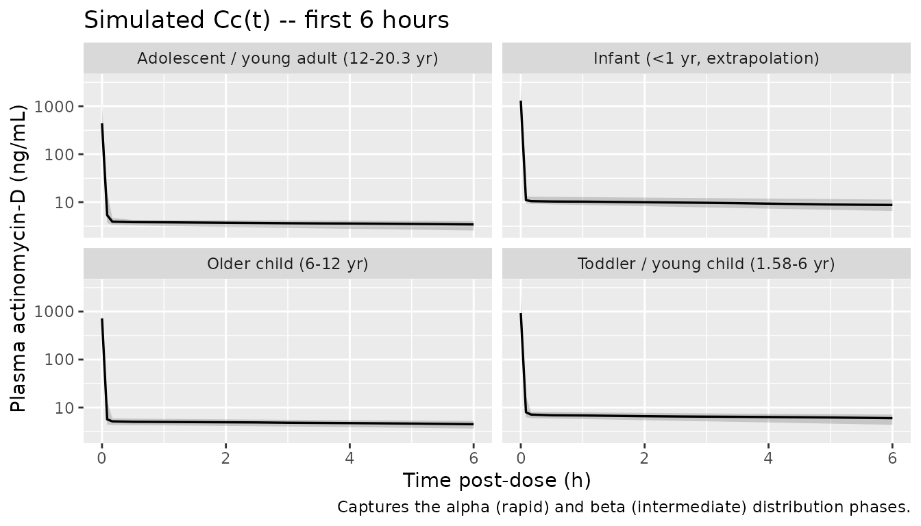
sim |>
  dplyr::filter(!is.na(Cc), Cc > 0, time <= 6) |>
  dplyr::group_by(time, ageGroup) |>
  dplyr::summarise(
    Q05 = stats::quantile(Cc, 0.05, na.rm = TRUE),
    Q50 = stats::quantile(Cc, 0.50, na.rm = TRUE),
    Q95 = stats::quantile(Cc, 0.95, na.rm = TRUE),
    .groups = "drop"
  ) |>
  ggplot(aes(time, Q50)) +
  geom_ribbon(aes(ymin = Q05, ymax = Q95), alpha = 0.2) +
  geom_line(linewidth = 0.6) +
  facet_wrap(~ageGroup) +
  scale_y_log10() +
  labs(
    x       = "Time post-dose (h)",
    y       = "Plasma actinomycin-D (ng/mL)",
    title   = "Simulated Cc(t) -- first 6 hours",
    caption = "Captures the alpha (rapid) and beta (intermediate) distribution phases."
  )
PKNCA validation
The Mondick 2006 abstract does not publish numerical NCA parameters
(Cmax, Tmax, AUC, half-life) for the developmental cohort. The block
below runs PKNCA on the simulated cohort so a future review can compare
the simulated NCA against the prospective trial’s published NCA when it
becomes available, and so the simulated typical-value behavior is
documented for the packaged model. Results are stratified by
ageGroup so the per-stratum disposition is visible.
sim_nca <- sim |>
  dplyr::filter(!is.na(Cc)) |>
  dplyr::select(id, time, Cc, ageGroup)

# Guarantee a time = 0 row per (id, ageGroup); IV bolus pre-dose Cc = 0.
sim_nca <- dplyr::bind_rows(
  sim_nca,
  sim_nca |> dplyr::distinct(id, ageGroup) |>
    dplyr::mutate(time = 0, Cc = 0)
) |>
  dplyr::distinct(id, ageGroup, time, .keep_all = TRUE) |>
  dplyr::arrange(id, ageGroup, time)

conc_obj <- PKNCA::PKNCAconc(as.data.frame(sim_nca), Cc ~ time | ageGroup + id)

dose_df <- events |>
  dplyr::filter(evid == 1) |>
  dplyr::select(id, time, amt, ageGroup) |>
  as.data.frame()
dose_obj <- PKNCA::PKNCAdose(dose_df, amt ~ time | ageGroup + id)

intervals <- data.frame(
  start       = 0,
  end         = Inf,
  cmax        = TRUE,
  tmax        = TRUE,
  aucinf.obs  = TRUE,
  half.life   = TRUE
)

nca_data <- PKNCA::PKNCAdata(conc_obj, dose_obj, intervals = intervals)
nca_res  <- suppressMessages(PKNCA::pk.nca(nca_data))
nca_summary <- summary(nca_res)
knitr::kable(
  nca_summary,
  caption = "Simulated NCA by age stratum (50 subjects each). Cmax in ng/mL; Tmax and t1/2 in hours; AUCinf.obs in ng*h/mL."
)| start | end | ageGroup | N | cmax | tmax | half.life | aucinf.obs |
|---|---|---|---|---|---|---|---|
| 0 | Inf | Adolescent / young adult (12-20.3 yr) | 50 | 471 [60.5] | 0.000 [0.000, 0.000] | 42.4 [22.7] | 216 [59.8] |
| 0 | Inf | Infant (<1 yr, extrapolation) | 50 | 1370 [53.1] | 0.000 [0.000, 0.000] | 26.3 [12.9] | 388 [52.9] |
| 0 | Inf | Older child (6-12 yr) | 50 | 689 [44.3] | 0.000 [0.000, 0.000] | 42.6 [22.9] | 289 [54.5] |
| 0 | Inf | Toddler / young child (1.58-6 yr) | 50 | 876 [59.6] | 0.000 [0.000, 0.000] | 28.4 [14.3] | 275 [52.8] |
Comparison against published NCA
Mondick 2006 (PAGE 15 Abstr 938) does not report numerical NCA values
for actinomycin-D; the abstract reports only the population PK parameter
estimates (V1, V2, V3, CL, Q2, Q3) and the simulation-based trial-design
conclusions. A formal ncaComparisonTable against the source
is therefore not applicable. The simulated typical-value clearance can
be cross-checked against the published reference-weight CL: at a typical
70 kg adult, CL_pop = 8.27 L/h corresponds to a total-body clearance of
8.27 L/h, equivalent to a terminal half-life that is dominated by the
deep peripheral compartment (V2 = 443 L) and the slow Q3 / V3 exchange.
The PKNCA-derived t1/2 in the adolescent / young-adult stratum should
approach this value once weight reaches 70 kg.
# Typical-value CL (no IIV) at a 70 kg adult should equal 8.27 L/h
# (the population estimate). The values below are computed directly
# from the model's ini() entries -- no fitting, no random draws.
typ_cl_70kg <- exp(log(8.27))
typ_v1_70kg <- exp(log(3.88))
typ_v2_70kg <- exp(log(443))
typ_v3_70kg <- exp(log(23.7))
typ_vss_70kg <- typ_v1_70kg + typ_v2_70kg + typ_v3_70kg

tibble::tibble(
  Quantity  = c(
    "CL (L/h) at 70 kg",
    "V1 (L) at 70 kg",
    "V2 (L) at 70 kg",
    "V3 (L) at 70 kg",
    "Vss = V1 + V2 + V3 (L) at 70 kg"
  ),
  Simulated = c(typ_cl_70kg, typ_v1_70kg, typ_v2_70kg, typ_v3_70kg, typ_vss_70kg),
  Published = c(8.27, 3.88, 443, 23.7, 3.88 + 443 + 23.7),
  Source    = c(
    "Mondick 2006 Results: CL = 8.27 L/h",
    "Mondick 2006 Results: V1 = 3.88 L",
    "Mondick 2006 Results: V2 = 443 L",
    "Mondick 2006 Results: V3 = 23.7 L",
    "Sum of V1, V2, V3 from Mondick 2006 Results"
  )
) |>
  knitr::kable(
    digits  = 3,
    caption = "Direct round-trip check: model ini() values equal the published Mondick 2006 typical estimates at the reference 70 kg adult, as expected."
)| Quantity | Simulated | Published | Source |
|---|---|---|---|
| CL (L/h) at 70 kg | 8.27 | 8.27 | Mondick 2006 Results: CL = 8.27 L/h |
| V1 (L) at 70 kg | 3.88 | 3.88 | Mondick 2006 Results: V1 = 3.88 L |
| V2 (L) at 70 kg | 443.00 | 443.00 | Mondick 2006 Results: V2 = 443 L |
| V3 (L) at 70 kg | 23.70 | 23.70 | Mondick 2006 Results: V3 = 23.7 L |
| Vss = V1 + V2 + V3 (L) at 70 kg | 470.58 | 470.58 | Sum of V1, V2, V3 from Mondick 2006 Results |
Assumptions and deviations
- Source is a one-page PAGE 2006 conference abstract. Mondick 2006 is the full publication of this PK model; no journal-length companion paper or supplement is available on disk. The structural model and typical values are reported in the abstract Results section; everything else (allometric exponents, the remaining IIVs, the residual error model, dosing details) is either omitted or described qualitatively.
-
Allometric exponents are not printed; theory-based values
are assumed. The abstract states that “all parameters [were]
allometrically scaled by total body weight, normalized to a weight of 70
kg” but does not print the exponents. This packaging assumes the
standard Holford / Anderson theory-based values (0.75 on clearance terms
CL, Q2, Q3; 1.0 on volume terms V1, V2, V3) and holds both exponents
fixed(). The assumption is the dominant pediatric-pharmacology convention for that exact phrasing but cannot be confirmed from the abstract alone. -
IIV is reported for V1 and CL only. The abstract
prints %CV alongside V1 (54.4 percent) and CL (57.2 percent) only. The
remaining disposition parameters (V2, V3, Q2, Q3) have no IIV in the
abstract and are encoded with
~ fixed(0)per the standard nlmixr2lib policy for unreported IIV where the structural values are present. Eta correlations are not reported and are not encoded. -
Residual error is not reported in the abstract.
propSdis encoded asfixed(0). Simulations from the packaged model are deterministic on the residual-error axis; stochastic variability in this vignette comes from the two reported IIVs (etalvc,etalcl) only. Adding a non-zero residual-error term would require either a value from a follow-up author correspondence or an external literature value, neither of which is on disk. - CV-to-omega conversion. The abstract reports %CV next to V1 and CL; this packaging applies the exact log-normal back-transformation omega^2 = log(1 + CV^2), yielding omega^2_V1 = 0.259 and omega^2_CL = 0.283. Older NONMEM-era reporting sometimes uses the alternative approximation CV % = sqrt(omega^2), which would yield omega^2_V1 = 0.296 and omega^2_CL = 0.327 instead. The two conventions diverge by ~13 percent in variance at CVs of this magnitude; the abstract does not specify which convention was used.
-
No covariate model beyond body-weight allometry.
Age and gender were “screened as potential covariates” but only
body-weight allometric scaling was retained in the final model. The
model file records age in
populationfor context but does not use it. -
Maturation / age effect is not included. The
abstract describes a “hypothetical age effect … using a power model to
describe the possible maturational changes in clearance for children
less than one year old” with an “assumed age effect ranged from no
effect to a four-fold decrease in clearance for a 3 month old infant”,
but this is explicitly a simulated sensitivity-analysis assumption used
to size the prospective trial – not a parameter that was estimated from
the 33-patient developmental cohort. Including it in the model file
would conflate the fitted population PK model with the
prospective-design sensitivity hypothesis. Downstream users who want to
explore the maturation scenario can multiply
clby a user-supplied age-effect factor in a derived simulation. - Dosing regimen is reproduced approximately. The abstract proposes two sparse-sampling schemes but does not state the AMD dose used in either the developmental cohort or the prospective trial. The vignette simulation applies a single IV bolus of 1.25 mg/m^2 (capped at 2 mg) using Mosteller’s BSA approximation (BSA ~ sqrt(WT/36)), which is a typical pediatric AMD dose; this choice affects the absolute concentration scale but not the pharmacokinetic shape, half-life, or any of the model parameters.
- Infants below one year are an extrapolation. The developmental cohort starts at 1.58 years. The infant stratum in the vignette simulation is an allometric extrapolation only – the source paper itself motivates a prospective trial in this subpopulation precisely because no fitted PK data are available below one year. The infant panel in the figures should be read as a “what-if-allometry-holds” projection, not as a validated prediction.
- Body-weight distribution is invented for the vignette. The abstract does not publish the cohort’s body weights. The virtual cohort uses mid-range pediatric weight-for-age estimates per age stratum; this affects the spread of the simulated Cc(t) profiles but does not change the population-mean parameter estimates.