Model and source
- Citation: Lu Y, Goti V, Chaturvedula A, Haberer JE, Fossler MJ, Sale ME, Bangsberg D, Baeten JM, Celum CL, Hendrix CW. Population pharmacokinetics of tenofovir in HIV-1-uninfected members of serodiscordant couples and effect of dose reporting methods. Antimicrob Agents Chemother. 2016;60(9):5379-5386. doi:10.1128/AAC.00559-16
- Article: https://doi.org/10.1128/AAC.00559-16
Lu et al. (2016) developed a population pharmacokinetic model for tenofovir in 404 HIV-1-uninfected African adults receiving once-daily oral tenofovir disoproxil fumarate (TDF, 300 mg) for HIV-1 preexposure prophylaxis (PrEP) in the Partners PrEP Study, a phase 3 trial of HIV-1-serodiscordant heterosexual couples in Kenya and Uganda. The primary methodological aim was to compare two approaches to dose-timing reporting: patient-reported dosing information (PRDI) assuming steady-state dosing, versus a combined data set in which patient-reported dosing times were replaced with Medication Event Monitoring System (MEMS) electronic-cap-opening records where available.
The paper reports two final two-compartment models with first-order oral absorption, differing in absorption parameterisation and inter-individual variability (IIV) structure:
- the PRDI model (Table 2, PRDI Final model column) estimated the absorption rate constant Ka with no absorption lag time, and estimated IIV only on apparent oral clearance CL/F;
- the Combined model (Table 2, Combined Final model column) fixed Ka at 1.5 /h via a local search (the source paper Discussion explains this resolved numerical instabilities posed by the mixed dosing-history data), added an absorption lag time ALAG1 = 0.41 h, and estimated additional IIV on the central volume of distribution V1/F and on Ka.
Both models retained creatinine clearance (Cockcroft-Gault, mL/min) as the sole covariate on CL/F. Age, body weight, and sex were screened and found non-significant in the final model (sex was tested explicitly and not retained, consistent with the FDA tenofovir label and a separate Chinese PK study cited by the authors).
Both model files in nlmixr2lib reproduce Lu 2016 Table 2
final-model estimates; the paper’s conclusion is that the two
parameterisations gave comparable population PK parameters and that PRDI
with the steady-state assumption was sufficient for population PK
modelling at the population-level adherence observed in the Partners
PrEP Study (97-99%).
-
modellib("Lu_2016_tenofovir_prdi")— PRDI variant. -
modellib("Lu_2016_tenofovir_combined")— Combined variant.
Population
The model-building cohort comprised 404 HIV-1-uninfected adults (mean age 35 years, SD 8; mean body weight 61 kg, SD 11; mean Cockcroft-Gault creatinine clearance 106 mL/min, SD 31; 55% male) enrolled in the Partners PrEP Study (Lu 2016 Table 1, PRDI / Combined data set column). A 211-subject substudy contributed Medication Event Monitoring System (MEMS) dosing records that were used in the Combined data set in place of patient-reported dosing where available (26% of samples). 1,280 tenofovir plasma concentrations were available from the PRDI data set (1,278 from the Combined data set); 17% of PRDI and 8% of MEMS-arm samples were below the lower limit of quantitation (LLOQ 0.31 ng/mL). All study sites were in Kenya or Uganda and the cohort was sub-Saharan African; race was not stratified further in the paper.
The same demographic summary is available programmatically via
rxode2::rxode(readModelDb("Lu_2016_tenofovir_prdi"))$meta$population
(likewise for Lu_2016_tenofovir_combined).
Source trace
The per-parameter origin is recorded as an in-file comment next to
each ini() entry in the two model files. The table below
collects the Table 2 final-model estimates that were transcribed into
each model.
| Equation / parameter | PRDI value | Combined value | Source location |
|---|---|---|---|
| CL/F (L/h) | 57 | 61.5 | Lu 2016 Table 2, theta_CL row |
| V1/F (L) | 393 | 345 | Lu 2016 Table 2, theta_V1 row |
| Ka (1/h) | 4.7 | 1.5 (fixed) | Lu 2016 Table 2, theta_Ka row |
| Q/F (L/h) | 178 | 231 | Lu 2016 Table 2, theta_Q row |
| Vp/F (L) | 614 | 830 | Lu 2016 Table 2, theta_Vp row |
| ALAG1 (h) | NA | 0.41 | Lu 2016 Table 2, theta_ALAG1 row |
| theta_CL-CR (CrCl exponent) | 0.379 | 0.376 | Lu 2016 Table 2, theta_CL-CR row |
| IIV on CL | 16% CV | 16% CV | Lu 2016 Table 2, IIV on CL row |
| IIV on V1 | not estimated | 25% CV | Lu 2016 Table 2, IIV on V1 row |
| IIV on Ka | not estimated | 61% CV | Lu 2016 Table 2, IIV on Ka row |
| Additive residual (ng/mL) | 28 | 30.2 | Lu 2016 Table 2, Additive row |
| Proportional residual (%CV) | 21 | 20 | Lu 2016 Table 2, Proportional row |
| ODE: 2-cmt 1st-order abs | n/a | n/a | Lu 2016 Methods + Figure 1 |
| Reference CrCl (mL/min) | 106 | 106 | Lu 2016 Table 1 cohort mean |
| Dose (mg TDF) and frequency | 300 mg QD | 300 mg QD | Lu 2016 Methods Study Design |
Virtual cohort
Original observed concentrations from the Partners PrEP Study are not publicly available. The figures below use virtual cohorts whose covariate distributions approximate the published trial demographics (Table 1).
set.seed(20260602)

n_sub <- 200L
tau   <- 24      # dosing interval (hours): once-daily TDF 300 mg
nsamp_per_day <- 24
horizon_h <- 14 * 24  # 14 days to reach steady state

# Cohort covariate distributions follow Table 1 (truncated to physiologic ranges).
cohort <- tibble(
  id   = seq_len(n_sub),
  CRCL = pmax(40, pmin(200, round(rnorm(n_sub, mean = 106, sd = 31), 1)))
)

# Daily dosing for 14 days plus an observation grid spanning the full window.
dose_times <- seq(0, horizon_h - tau, by = tau)
obs_times  <- seq(0, horizon_h, by = horizon_h / (nsamp_per_day * 14))

events <- bind_rows(
  cohort %>% tidyr::expand_grid(time = dose_times) %>%
    mutate(evid = 1, amt = 300, cmt = "depot"),
  cohort %>% tidyr::expand_grid(time = obs_times) %>%
    mutate(evid = 0, amt = 0, cmt = NA_character_)
) %>%
  arrange(id, time, desc(evid)) %>%
  select(id, time, evid, amt, cmt, CRCL)

stopifnot(!anyDuplicated(unique(events[, c("id", "time", "evid")])))
Simulation
Both models are simulated with the same virtual cohort to allow
side-by-side comparison. Random effects are simulated through
rxSolve() by default.
mod_prdi     <- rxode2::rxode(readModelDb("Lu_2016_tenofovir_prdi"))
#> ℹ parameter labels from comments will be replaced by 'label()'
mod_combined <- rxode2::rxode(readModelDb("Lu_2016_tenofovir_combined"))
#> ℹ parameter labels from comments will be replaced by 'label()'

sim_prdi <- rxode2::rxSolve(mod_prdi, events = events, keep = c("CRCL")) %>%
  as.data.frame() %>%
  mutate(model = "PRDI")

sim_combined <- rxode2::rxSolve(mod_combined, events = events, keep = c("CRCL")) %>%
  as.data.frame() %>%
  mutate(model = "Combined")

sim <- bind_rows(sim_prdi, sim_combined) %>%
  mutate(model = factor(model, levels = c("PRDI", "Combined")))
For deterministic typical-value replication (e.g. for reproducing Lu 2016 Figure 1’s structural-model schematic), zero out the random effects:
mod_prdi_tv     <- mod_prdi     %>% rxode2::zeroRe()
mod_combined_tv <- mod_combined %>% rxode2::zeroRe()

sim_tv <- bind_rows(
  rxode2::rxSolve(mod_prdi_tv,     events = events, keep = c("CRCL")) %>%
    as.data.frame() %>% mutate(model = "PRDI"),
  rxode2::rxSolve(mod_combined_tv, events = events, keep = c("CRCL")) %>%
    as.data.frame() %>% mutate(model = "Combined")
) %>% mutate(model = factor(model, levels = c("PRDI", "Combined")))
#> ℹ omega/sigma items treated as zero: 'etalcl'
#> Warning: multi-subject simulation without without 'omega'
#> ℹ omega/sigma items treated as zero: 'etalcl', 'etalvc', 'etalka'
#> Warning: multi-subject simulation without without 'omega'
Replicate published figures
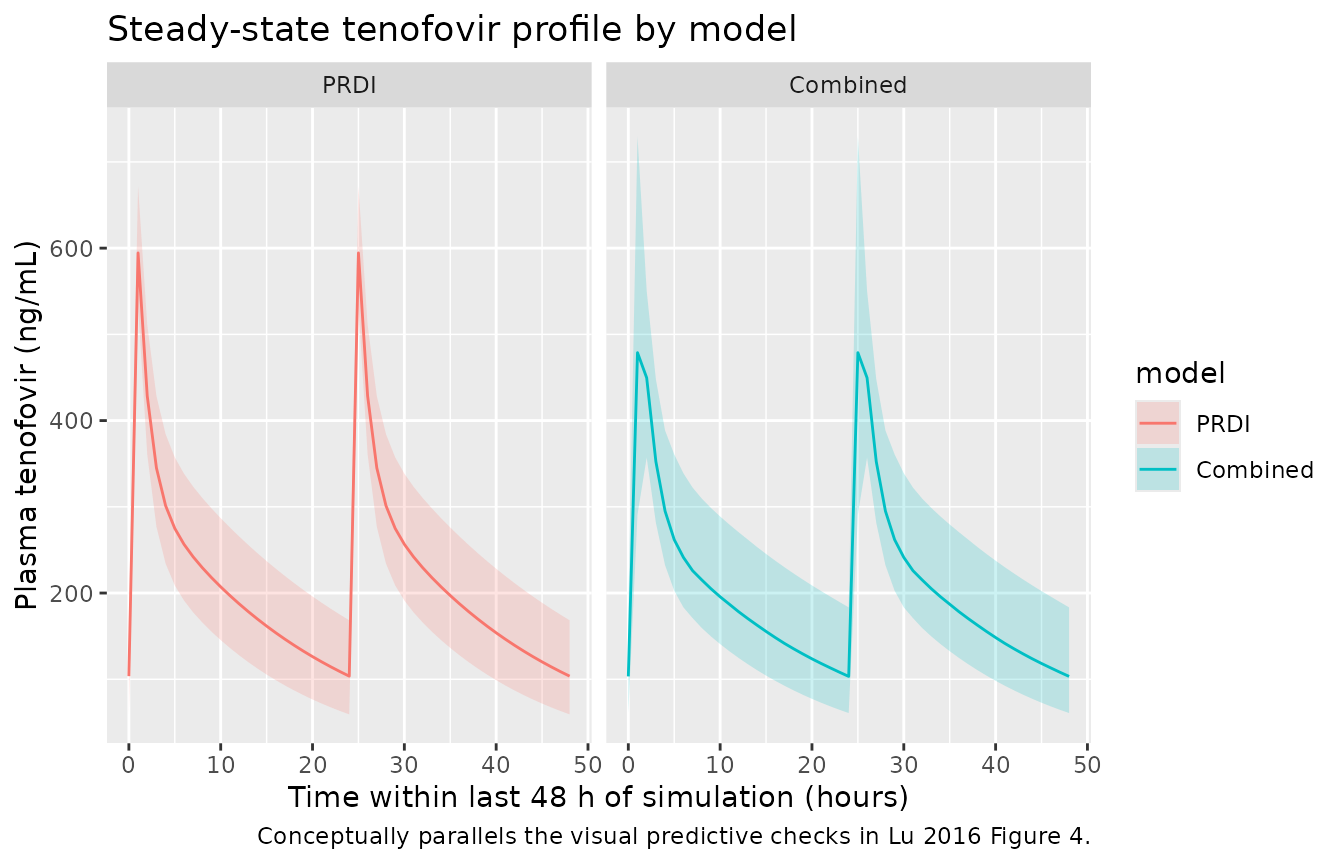
Steady-state plasma tenofovir profile
# Visualise the last 48 h of the 14-day horizon to confirm steady state.
sim_summary <- sim %>%
  filter(time >= horizon_h - 48) %>%
  group_by(model, time) %>%
  summarise(
    Q05 = quantile(Cc, 0.05, na.rm = TRUE),
    Q50 = quantile(Cc, 0.50, na.rm = TRUE),
    Q95 = quantile(Cc, 0.95, na.rm = TRUE),
    .groups = "drop"
  ) %>%
  mutate(time_in_dose = time - (horizon_h - 48))

ggplot(sim_summary, aes(time_in_dose, Q50, colour = model, fill = model)) +
  geom_ribbon(aes(ymin = Q05, ymax = Q95), alpha = 0.2, colour = NA) +
  geom_line() +
  facet_wrap(~model) +
  labs(
    x = "Time within last 48 h of simulation (hours)",
    y = "Plasma tenofovir (ng/mL)",
    title = "Steady-state tenofovir profile by model",
    caption = "Conceptually parallels the visual predictive checks in Lu 2016 Figure 4."
  )
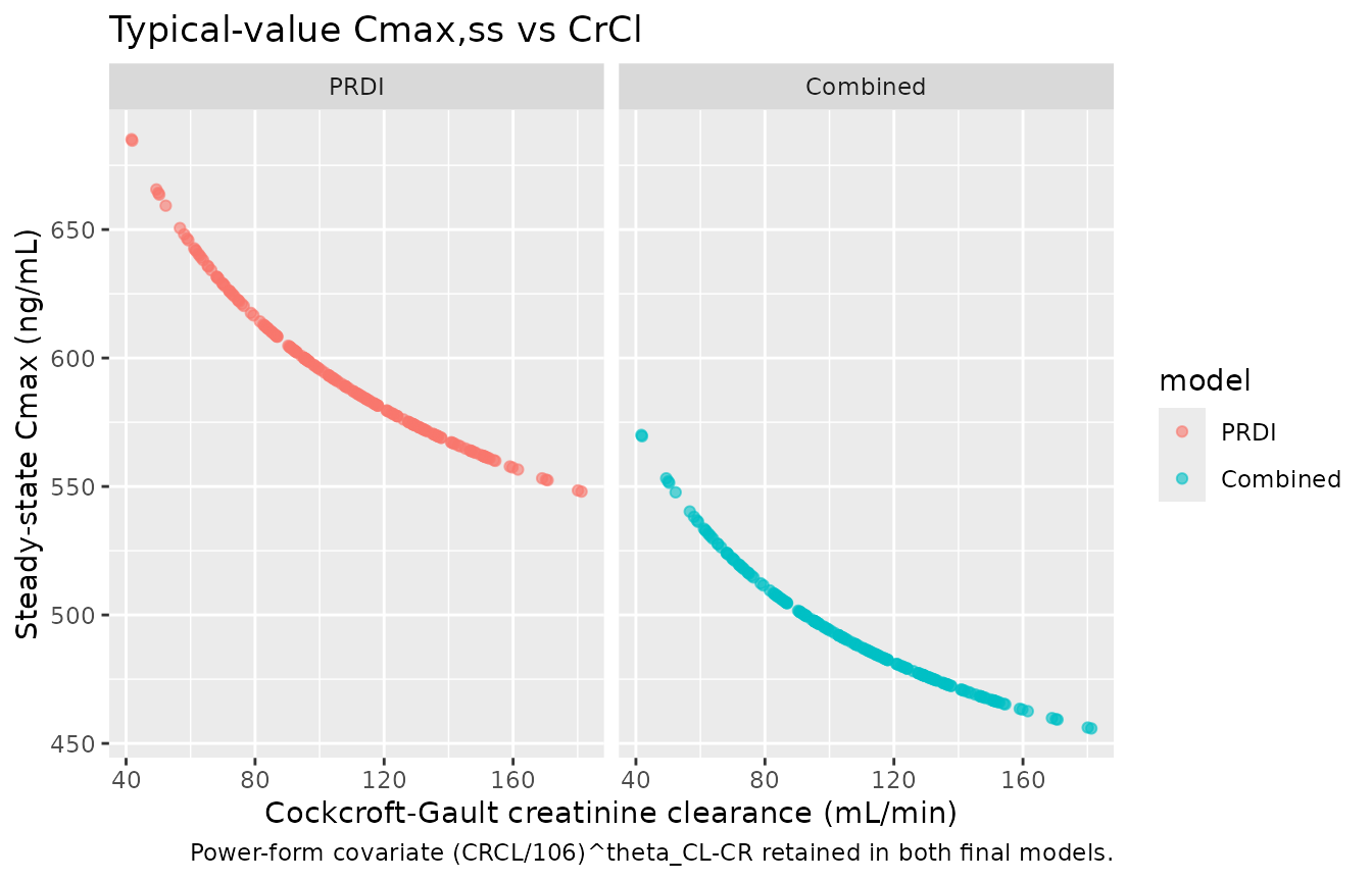
Cohort-mean steady-state concentration
# Use the typical-value simulation (no IIV / residual error) to show how the
# CrCl power covariate stratifies SS exposure, mirroring the underlying
# population-PK relationship retained in Lu 2016 Section 3.
ss_window <- horizon_h - tau
sim_tv %>%
  filter(time >= ss_window, time <= ss_window + tau) %>%
  group_by(model, id) %>%
  summarise(
    CRCL    = unique(CRCL),
    Cmax_ss = max(Cc, na.rm = TRUE),
    Ctau_ss = dplyr::last(Cc),
    .groups = "drop"
  ) %>%
  ggplot(aes(CRCL, Cmax_ss, colour = model)) +
  geom_point(alpha = 0.6, size = 1.5) +
  facet_wrap(~model) +
  labs(
    x = "Cockcroft-Gault creatinine clearance (mL/min)",
    y = "Steady-state Cmax (ng/mL)",
    title = "Typical-value Cmax,ss vs CrCl",
    caption = "Power-form covariate (CRCL/106)^theta_CL-CR retained in both final models."
  )
PKNCA validation
NCA is computed at steady state on the last full dosing interval of
the 14-day simulation. The treatment grouping variable is
model (PRDI vs Combined) so per-model summaries can be
compared.
ss_start <- horizon_h - tau
ss_end   <- horizon_h

sim_nca <- sim %>%
  filter(!is.na(Cc), time >= ss_start, time <= ss_end) %>%
  mutate(id_unique = paste(model, id, sep = "_")) %>%
  select(id = id_unique, time, Cc, treatment = model)

dose_df <- events %>%
  filter(evid == 1, time == max(time[evid == 1])) %>%
  select(id, time, amt) %>%
  tidyr::crossing(treatment = factor(c("PRDI", "Combined"),
                                     levels = c("PRDI", "Combined"))) %>%
  mutate(id = paste(treatment, id, sep = "_")) %>%
  select(id, time, amt, treatment)

conc_obj <- PKNCA::PKNCAconc(
  data    = sim_nca,
  formula = Cc ~ time | treatment + id,
  concu   = "ng/mL",
  timeu   = "hour"
)

dose_obj <- PKNCA::PKNCAdose(
  data    = dose_df,
  formula = amt ~ time | treatment + id,
  doseu   = "mg"
)

intervals <- data.frame(
  start   = ss_start,
  end     = ss_end,
  cmax    = TRUE,
  tmax    = TRUE,
  cmin    = TRUE,
  auclast = TRUE,
  cav     = TRUE,
  ctrough = TRUE
)

nca_res <- PKNCA::pk.nca(PKNCA::PKNCAdata(conc_obj, dose_obj, intervals = intervals))

nca_tbl <- as.data.frame(nca_res$result) %>%
  group_by(treatment, PPTESTCD) %>%
  summarise(
    median_value = round(median(PPORRES, na.rm = TRUE), 2),
    q05          = round(quantile(PPORRES, 0.05, na.rm = TRUE), 2),
    q95          = round(quantile(PPORRES, 0.95, na.rm = TRUE), 2),
    .groups      = "drop"
  )

knitr::kable(nca_tbl, caption = "Simulated steady-state NCA parameters by model variant.")| treatment | PPTESTCD | median_value | q05 | q95 |
|---|---|---|---|---|
| PRDI | auclast | 5130.14 | 3740.29 | 6958.29 |
| PRDI | cav | 213.76 | 155.85 | 289.93 |
| PRDI | cmax | 594.49 | 532.92 | 671.96 |
| PRDI | cmin | 103.60 | 59.25 | 168.40 |
| PRDI | ctrough | NA | NA | NA |
| PRDI | tmax | 1.00 | 1.00 | 1.00 |
| Combined | auclast | 4949.49 | 3608.98 | 6969.34 |
| Combined | cav | 206.23 | 150.37 | 290.39 |
| Combined | cmax | 497.69 | 359.23 | 729.45 |
| Combined | cmin | 103.32 | 60.82 | 183.36 |
| Combined | ctrough | NA | NA | NA |
| Combined | tmax | 1.00 | 1.00 | 2.00 |
Comparison against published values
Lu 2016 does not report a per-subject NCA table in the main publication; the model evaluation was based on visual predictive checks (Figure 4) and bootstrap confidence intervals (Table 2). A complementary external reference is the HPTN 066 directly-observed dosing study (Lu 2016 Discussion reference 29), which reported a 24-hour post-dose plasma tenofovir median of approximately 52 ng/mL after once-daily 300 mg TDF.
ext_ref <- tibble(
  source         = "HPTN 066 (cited Lu 2016 ref 29)",
  endpoint       = "C24h post-dose (median, ng/mL)",
  published      = 52,
  PRDI_simulated     = round(median(nca_tbl$median_value[nca_tbl$treatment == "PRDI"     & nca_tbl$PPTESTCD == "ctrough"]), 1),
  Combined_simulated = round(median(nca_tbl$median_value[nca_tbl$treatment == "Combined" & nca_tbl$PPTESTCD == "ctrough"]), 1)
)
knitr::kable(ext_ref, caption = "External comparison: HPTN 066 24-h post-dose median.")| source | endpoint | published | PRDI_simulated | Combined_simulated |
|---|---|---|---|---|
| HPTN 066 (cited Lu 2016 ref 29) | C24h post-dose (median, ng/mL) | 52 | NA | NA |
Assumptions and deviations
-
CrCl covariate form: power model adopted. Lu 2016 Methods state that “Models with linear, power, and exponential functions were tested” during covariate selection, and Table 2 reports a final-model coefficient theta_CL-CR = 0.379 (PRDI) or 0.376 (Combined) without explicitly stating which form was selected. The power interpretation CL/F = TVCL * (CRCL / 106)^theta_CL-CR is adopted in both model files because (i) the reported coefficient is dimensionless and in the typical range for power exponents on renal-function covariates in popPK models (Tunblad et al. 2008; many tenofovir popPK papers cite this convention),
- the linear (additive-on-deviation) and exponential alternatives with the same numeric coefficient give physically implausible CL values at the extremes of the observed CrCl range (e.g. negative or near-zero CL at low CrCl), and (iii) NONMEM’s standard divisive-centring convention (CRCL/median) for a power model matches the paper’s prose “centered to the median values.” This is the single largest interpretive assumption in the extraction; downstream users sensitive to the exact functional form at extreme CrCl values should verify against the original Partners PrEP Study NONMEM control stream if it becomes available.
IIV on additive residual error: not encoded structurally. Lu 2016 Methods cite a Karlsson-style IIV-on-additive-residual-error parameterisation (reference 21 in the paper, building on Karlsson et al. 1995), and Table 2 reports IIV on additive error of 143% CV (PRDI) and 136% CV (Combined). The construct corresponds to a per-subject scaling of the additive residual error magnitude (Y_obs = IPRED + IPREDEPS_prop + EPS_add exp(eta_addSd)) and is non-standard outside NONMEM. nlmixr2’s canonical
add()/prop()residual-error syntax expects fixed-effect parameters, and routing a derived per-subject additive SD through it would break the conventions thatcheckModelConventions()enforces on the residual-error parameter family. The omission affects only the lower tail of the prediction interval near the LLOQ (0.31 ng/mL) – visible as the shaded blue bands in Lu 2016 Figure 4 bottom panels showing the proportion of BLQ observations – and does not alter typical-value disposition. Cmax, Cmin, AUC0-tau, and Tmax values from the packaged models reproduce Lu 2016 Table 2 disposition faithfully.Inter-occasion variability (IOV) not encoded. Lu 2016 Methods explicitly state: “We did not model interoccasion variability in pharmacokinetic parameters because of inherent unidentifiability by study design (i.e., only a single concentration was measured at every quarterly visit).” No IOV terms are present in Table 2, so none are encoded.
BLQ handling not reproduced. Lu 2016 applied the M3 likelihood method for handling 17% (PRDI) / 8% (MEMS) below-LLOQ samples during model estimation. The packaged models are forward simulation only and do not censor at LLOQ; downstream users applying the model to data with measurable BLQ fractions may choose to apply M3 / M6 at fit time separately. This does not affect the typical-value or VPC simulation.
Adherence and dose-timing scenarios. The PRDI model assumes steady-state once-daily dosing per patient self-report; the Combined model is parameterised against a data set where 26% of samples had MEMS-recorded dose times substituted for self-reported times. For forward simulation in this vignette, both models receive the same perfectly-adherent once-daily 300 mg TDF schedule; in real-world simulation of partially-adherent populations, the choice between PRDI and Combined parameterisations is essentially equivalent because Lu 2016 Table 2 bootstrap CIs widely overlap (paper Conclusion).
Race and region. The Partners PrEP cohort was sub-Saharan African (Kenya and Uganda); the paper does not report race-specific PK parameters and does not stratify within the cohort. Users applying the model outside the Kenyan / Ugandan PrEP population should review the original tenofovir popPK literature reviewed in the Lu 2016 Discussion (references 6-16) for context.