Vancomycin (Ahmed 2024)
Source:vignettes/articles/Ahmed_2024_vancomycin.Rmd
Ahmed_2024_vancomycin.RmdModel and source
- Citation: Ahmed KA, Ibrahim A, Gonzalez D, Nur AO. Population Pharmacokinetics and Model-Based Dose Optimization of Vancomycin in Sudanese Adult Patients with Renal Impairment. Drug Des Devel Ther. 2024;18:81-95. doi:10.2147/DDDT.S432439
- Description: One-compartment intravenous population PK model for vancomycin in Sudanese adult inpatients, developed from routine therapeutic-drug-monitoring peak and trough concentrations at a single hospital in Khartoum. Clearance is a median-centered power function of creatinine clearance; volume of distribution carries no covariates. IMPORTANT: the CRCL column is NOT a conventional creatinine clearance in mL/min – the source computes it as Bjornson’s creatinine production rate divided by serum creatinine with the body-weight and 14.4 unit factors omitted, which deflates it about five-fold relative to a Cockcroft-Gault value; see covariateData$CRCL.
- Article: https://doi.org/10.2147/DDDT.S432439 (open access)
mod <- nlmixr2lib::modellib("Ahmed_2024_vancomycin")
mod
#> function() {
#>   description <- "One-compartment intravenous population PK model for vancomycin in Sudanese adult inpatients, developed from routine therapeutic-drug-monitoring peak and trough concentrations at a single hospital in Khartoum. Clearance is a median-centered power function of creatinine clearance; volume of distribution carries no covariates. IMPORTANT: the CRCL column is NOT a conventional creatinine clearance in mL/min -- the source computes it as Bjornson's creatinine production rate divided by serum creatinine with the body-weight and 14.4 unit factors omitted, which deflates it about five-fold relative to a Cockcroft-Gault value; see covariateData$CRCL."
#>   reference <- "Ahmed KA, Ibrahim A, Gonzalez D, Nur AO. Population Pharmacokinetics and Model-Based Dose Optimization of Vancomycin in Sudanese Adult Patients with Renal Impairment. Drug Des Devel Ther. 2024;18:81-95. doi:10.2147/DDDT.S432439"
#>   vignette <- "Ahmed_2024_vancomycin"
#>   units <- list(time = "h", dosing = "mg", concentration = "mg/L")
#>
#>   # Issue #482: what each ODE state holds, in what amount units, in what
#>   # biological matrix. Verified against the source: the single disposition
#>   # compartment holds vancomycin and is sampled as plasma concentration by the
#>   # EMIT immunoassay, calibration range 2-50 mg/L (Methods, "Vancomycin
#>   # Assay"). Both peak (1 h post-dose) and trough (30 min pre-dose) samples
#>   # inform the fit (Methods, "Dosing and Sample Collection").
#>   compartmentData <- list(
#>     central = list(analyte = "vancomycin", units = "mg", specimen = "plasma", verified = TRUE)
#>   )
#>
#>   covariateData <- list(
#>     CRCL = list(
#>       description = "Creatinine clearance as computed by Ahmed 2024 -- Bjornson creatinine production rate divided by serum creatinine, WITHOUT the body-weight multiplier or the 14.4 unit-conversion divisor of the published Bjornson method",
#>       units = "mL/min as labelled by the source; dimensionally (mg/kg/24 h)/(mg/dL) as actually computed",
#>       type = "continuous",
#>       reference_category = NULL,
#>       notes = paste(
#>         "READ THIS BEFORE SUPPLYING A CRCL VALUE TO THIS MODEL. Ahmed 2024 Methods, 'Patients and Data Collection',",
#>         "Equations 1-3: CLcr = Rcr / SCR, with Rcr(males) = 27 - 0.173 * age and Rcr(females) = 25 - 0.175 * age, both in",
#>         "mg/kg/24 h, and SCR in mg/dL. The published Bjornson method (Bjornsson TD, Clin Pharmacokinet 1979) completes the",
#>         "calculation as CrCl = Rcr * body weight / (SCr * 14.4) to reach mL/min; Ahmed 2024 states explicitly that 'the data",
#>         "lacked patient weight and height' and therefore stops at Rcr / SCr, while still labelling the column mL/min. The",
#>         "omitted factor is weight / 14.4, i.e. about 4.9 for a 70 kg adult, so this column runs roughly five-fold BELOW a",
#>         "Cockcroft-Gault or complete-Bjornson creatinine clearance for the same patient. The arithmetic is confirmed by the",
#>         "paper's own Table 1: the median male aged 65 with SCr 1.2 mg/dL gives (27 - 0.173 * 65) / 1.2 = 13.1, against the",
#>         "reported cohort median of 12.7. Because e_crcl_cl scales CL as a power of this column, feeding it a conventional",
#>         "mL/min creatinine clearance would inflate typical CL by about 4.9^0.49 = 2.2-fold. Users must reproduce the source's",
#>         "own calculation, not substitute a standard renal-function estimate. This also explains why a general medical-ward",
#>         "cohort appears almost uniformly renally impaired (median 12.7, IQR 5.52-25.78, range 1.4-107.5): the column is",
#>         "systematically deflated, not the cohort uniformly anuric. Enters CL as the median-centered power term",
#>         "(CRCL / 12.7)^0.49 -- see the model() block for why 12.7 is used and what the source does and does not print.",
#>         sep = " "
#>       ),
#>       source_name = "CLcr"
#>     )
#>   )
#>
#>   covariatesDataExcluded <- list(
#>     AGE = list(
#>       description = "Age at the time of the therapeutic-drug-monitoring episode",
#>       units = "years",
#>       type = "continuous",
#>       notes = paste(
#>         "Screened on CL and significant in univariate forward inclusion (Table 2 model 4, dOFV -16.9, p < 0.05) but not",
#>         "retained: once CLcr was in the model, adding age gave dOFV -0.06 (Table 2 model 8, p > 0.05). Age nonetheless enters",
#>         "the model indirectly, because it is an input to the Bjornson Rcr equations that generate CRCL.",
#>         sep = " "
#>       )
#>     ),
#>     CREAT = list(
#>       description = "Serum creatinine",
#>       units = "mg/dL",
#>       type = "continuous",
#>       notes = paste(
#>         "Screened on CL as log-transformed SCr and significant (Table 2 model 2, dOFV -43.73, p < 0.05), but CLcr gave the",
#>         "larger drop in both OFV (-49.69) and BSV on CL (omega 0.46 versus 0.49), so the CLcr model was selected as final",
#>         "(Results, 'Model Development'). The two are not independent -- SCr is the denominator of the CRCL calculation.",
#>         "Cohort median 1.2 mg/dL (IQR 0.7-2.5, range 0.2-9.5; Table 1).",
#>         sep = " "
#>       )
#>     ),
#>     ALB = list(
#>       description = "Serum albumin",
#>       units = "g/dL",
#>       type = "continuous",
#>       notes = paste(
#>         "Screened on both V (Table 2 model 6, dOFV -0.86) and CL (model 7, dOFV -0.30) and rejected at p > 0.05 in each case;",
#>         "also rejected when added to the CLcr model (model 10, dOFV -1.07). Cohort median 2.5 g/dL (IQR 2.1-2.9,",
#>         "range 1.4-4.1; Table 1). Reported here in the source's g/dL, not the canonical register unit g/L.",
#>         sep = " "
#>       )
#>     ),
#>     BUN = list(
#>       description = "Blood urea nitrogen",
#>       units = "mg/dL",
#>       type = "continuous",
#>       notes = paste(
#>         "Screened on CL and significant in univariate forward inclusion (Table 2 model 5, dOFV -28.84, p < 0.05) but not",
#>         "retained once CLcr was in the model (Table 2 model 9, dOFV -0.34, p > 0.05). Cohort median 52 mg/dL",
#>         "(IQR 26.1-89, range 5-215; Table 1, where it is headed 'Blood urea').",
#>         sep = " "
#>       )
#>     ),
#>     SEXF = list(
#>       description = "Female sex indicator",
#>       units = NULL,
#>       type = "categorical",
#>       notes = paste(
#>         "Screened on CL. The Discussion reports that adding sex to CL reduced the OFV by 6.03 points (p > 0.05) at the forward",
#>         "step and that it was removed at backward elimination, so it does not appear in Table 2 at all and no coefficient is",
#>         "published. Cohort 66 male / 33 female (Table 1). As with age, sex enters indirectly: it selects between the two",
#>         "Bjornson Rcr equations that generate CRCL.",
#>         sep = " "
#>       )
#>     )
#>   )
#>
#>   population <- list(
#>     species = "human",
#>     n_subjects = 99L,
#>     n_observations = 194L,
#>     n_studies = 1L,
#>     age_range = "18-90 years; median 65 (IQR 50-75) (Table 1)",
#>     age_median = "65 years",
#>     weight_range = "NOT RECORDED. Ahmed 2024 states that patient weight and height were absent from the medical records, which is why the Cockcroft-Gault equation could not be used and why the CRCL column omits its weight factor.",
#>     sex_female_pct = 33,
#>     race_ethnicity = "Not reported beyond nationality; single-country cohort of Sudanese adults. The paper motivates the study by noting that no vancomycin population PK information existed for Sudanese patients.",
#>     disease_state = "Adult inpatients receiving intravenous vancomycin at a single hospital. Patients under 18 years, pregnant patients, and patients on renal replacement therapy were excluded, so the model carries no information about dialysis. As reported by the source the cohort is dominated by renal impairment (median CLcr 12.7), but see covariateData$CRCL: the renal-function column is computed without its weight and unit factors and is therefore about five-fold deflated relative to a conventional creatinine clearance, so the apparent severity of impairment is partly an artefact of the covariate definition.",
#>     renal_function = "CLcr median 12.7 (IQR 5.52-25.78, range 1.4-107.5) in the source's own units (Table 1); serum creatinine median 1.2 mg/dL (IQR 0.7-2.5, range 0.2-9.5)",
#>     dose_range = "500-1000 mg intravenously every 12 h, infused over 60 min (Methods, 'Dosing and Sample Collection'); administered one to two times per day (Results, 'Patient Characteristics')",
#>     regions = "Sudan (Aliaa Specialist Hospital, Khartoum)",
#>     notes = "Retrospective single-centre observational cohort of patients treated between August 2016 and January 2019. 194 concentrations from 99 patients: 129 troughs (median 16.22 mg/L, IQR 11.1-26.53) drawn 30 min before the next dose and 65 peaks (median 29.55 mg/L, IQR 22.38-37.36) drawn 1 h after the dose, all from the fourth dose onwards. No samples were below the limit of quantitation. Assay: enzyme-multiplied immunoassay (EMIT), calibration range 2-50 mg/L. Fitted in MonolixSuite 2020R1 by SAEM. Baseline demographics are Table 1 of Ahmed 2024."
#>   )
#>
#>   ini({
#>     # All estimates are the "VALUE" (Monolix) column of Ahmed 2024 Table 3.
#>     # The model was fitted in MonolixSuite 2020R1 with log-normally distributed
#>     # individual parameters and an exponential BSV model (Methods, "Population
#>     # Pharmacokinetic Analysis"), so the population values below are entered on
#>     # the log scale.
#>
#>     lvc <- log(65);   label("Volume of distribution (L)")  # Ahmed 2024 Table 3, V_pop = 65 L (SE 6.12, RSE 9.41%; bootstrap median 66.78, 95% CI 62.49-71.18)
#>     lcl <- log(2.02); label("Clearance at the reference CRCL of 12.7 (L/h)")  # Ahmed 2024 Table 3, CL_pop = 2.02 L/h (SE 0.13, RSE 6.40%; bootstrap median 2.004, 95% CI 1.92-2.08)
#>
#>     # Covariate effect. Monolix names it beta_CL_logtCLcr: the slope of
#>     # log(CL) on the log-transformed, centered covariate logtCLcr, which is
#>     # identical to a power exponent on the centered ratio. See the model()
#>     # block for the two conflicting forms the paper prints and why the
#>     # centered one is used.
#>     e_crcl_cl <- 0.49; label("Power exponent on (CRCL / 12.7) for CL (unitless)")  # Ahmed 2024 Table 3, beta_CL_logtCLcr = 0.49 (SE 0.064, RSE 13%; bootstrap median 0.488, 95% CI 0.443-0.541)
#>
#>     # Inter-individual variability. Table 3 heads this block "Standard
#>     # Deviation of the Random Effects" and Monolix reports omega as an SD, so
#>     # the tabulated 0.39 / 0.46 are SDs of the log-normal etas and the
#>     # variances entered here are their squares. The 0.46 is corroborated in
#>     # the Results text, which tracks omega for CL falling "from 0.66 to 0.46"
#>     # when the CLcr effect was added.
#>     etalvc ~ 0.1521  # Ahmed 2024 Table 3, omega_V  = 0.39 (SD) -> variance 0.39^2 = 0.1521 (RSE 19.3%; bootstrap median 0.42, 95% CI 0.35-0.49)
#>     etalcl ~ 0.2116  # Ahmed 2024 Table 3, omega_Cl = 0.46 (SD) -> variance 0.46^2 = 0.2116 (RSE 12.5%; bootstrap median 0.45, 95% CI 0.41-0.49)
#>
#>     # Residual error. Both proportional and combined models were tested
#>     # (Methods); Table 3 reports only the proportional term b under the
#>     # heading "Standard Deviation of the Proportional Error", so the final
#>     # model is proportional-only. Monolix's proportional error model is
#>     # y = f + b * f * e with e ~ N(0, 1), so b maps directly onto propSd.
#>     propSd <- 0.28; label("Proportional residual error (fraction)")  # Ahmed 2024 Table 3, b = 0.28 (SE 0.023, RSE 8.26%; bootstrap median 0.28, 95% CI 0.26-0.29)
#>   })
#>
#>   model({
#>     # Covariate model on clearance.
#>     #
#>     #   CL_i = 2.02 * (CRCL / 12.7)^0.49 * exp(eta_CL)
#>     #   V_i  = 65 * exp(eta_V)
#>     #
#>     # THE CENTERING IS DELIBERATE AND THE PAPER PRINTS TWO CONFLICTING FORMS.
#>     # Ahmed 2024 Methods, "Population Pharmacokinetic Analysis" (p. 83), gives
#>     # the form that was actually fitted:
#>     #
#>     #   log(CL) = log(CL_pop) + beta_CL_logtCLcr * logtCLcr + eta_CL
#>     #   where   logtCLcr = log(CLcr / mean(CLcr))
#>     #   i.e.    CL = CL_pop * (CLcr / mean(CLcr))^beta_CL_logtCLcr * exp(eta_CL)
#>     #
#>     # Equation 5 on p. 85 and the Table 3 footnote both drop the denominator
#>     # and print CL = CL_pop * CLcr^0.49 * exp(eta). That uncentered form is
#>     # arithmetically impossible: it returns 2.02 * 12.7^0.49 = 6.9 L/h at the
#>     # cohort median and 2.02 * 54.5^0.49 = 14.2 L/h at the top simulated CLcr
#>     # group, against the 2.22 and 4.28 L/h that the paper's own Table 4 reports
#>     # as the median simulated clearance for those groups. The centered form is
#>     # therefore used, per the Methods equation.
#>     #
#>     # THE CENTERING CONSTANT ITSELF IS NOT PRINTED. The Methods define the
#>     # reference as mean(CLcr), a value the paper never reports; the only
#>     # central-tendency statistic published for the covariate is the median,
#>     # 12.7 (Table 1), which is the value used here. Back-solving the paper's
#>     # Table 4 median simulated clearances against CL_pop = 2.02 and the 0.49
#>     # exponent implies an effective reference of about 11.8 -- consistent to
#>     # within 2% across all five independent CLcr groups, and close to what a
#>     # Monolix log-transform centered on the mean of log(CLcr) would give (the
#>     # geometric mean, which for a right-skewed covariate sits just below the
#>     # median). Using 12.7 rather than that back-solved 11.8 leaves typical CL
#>     # about 4% low against Table 4 across the whole covariate range; that is
#>     # accepted here in preference to fitting a constant to the validation
#>     # target. The vignette quantifies the residual offset.
#>     cl <- exp(lcl + etalcl) * (CRCL / 12.7)^e_crcl_cl
#>     vc <- exp(lvc + etalvc)
#>
#>     # One-compartment disposition with first-order elimination. Ahmed 2024
#>     # Results, "Model Development": "A one-compartment model with first-order
#>     # elimination best characterized vancomycin's PK"; one- and two-compartment
#>     # models were both evaluated (Methods).
#>     kel <- cl / vc
#>
#>     # Doses enter the central compartment directly as intravenous infusions.
#>     # The source infused each dose over 60 min (Methods, "Dosing and Sample
#>     # Collection"); the infusion duration is a property of the event table
#>     # (rate / dur) rather than of the model.
#>     d/dt(central) <- -kel * central
#>
#>     # Vancomycin plasma concentration in mg/L (doses in mg, volume in L).
#>     Cc <- central / vc
#>     Cc ~ prop(propSd)
#>   })
#> }
#> <environment: 0x556799da3188>
Population
Ahmed 2024 is a retrospective, single-centre, observational cohort study at Aliaa Specialist Hospital, Khartoum, Sudan, covering patients treated with intravenous vancomycin between August 2016 and January 2019. Patients under 18 years, pregnant patients, and patients receiving renal replacement therapy were excluded.
The analysis dataset holds 194 concentrations from 99 adults (66 male / 33 female). Sampling was therapeutic-drug-monitoring driven and began with the fourth dose: 129 troughs drawn 30 min before the next dose (median 16.22 mg/L, IQR 11.1-26.53) and 65 peaks drawn 1 h after the dose (median 29.55 mg/L, IQR 22.38-37.36). No concentration fell below the limit of quantitation. The assay was an enzyme-multiplied immunoassay (EMIT) with a 2-50 mg/L calibration range. Usual dosing was 500-1000 mg every 12 h infused over 60 min. The model was fitted in MonolixSuite 2020R1 by SAEM.
Baseline characteristics (Ahmed 2024 Table 1):
| Characteristic | Median (IQR) | Range |
|---|---|---|
| Age (years) | 65 (50-75) | 18-90 |
| Serum creatinine (mg/dL) | 1.2 (0.7-2.5) | 0.2-9.5 |
| Serum albumin (g/dL) | 2.5 (2.1-2.9) | 1.4-4.1 |
| Blood urea (mg/dL) | 52 (26.1-89) | 5-215 |
| Creatinine clearance (source units) | 12.7 (5.52-25.78) | 1.4-107.5 |
| Trough concentration (mg/L) | 16.22 (11.1-26.53) | 4.41-53 |
| Peak concentration (mg/L) | 29.55 (22.38-37.36) | 11.5-62.5 |
Body weight and height were not recorded in the source medical files. That single data gap drives the most important caveat in this model, discussed next.
The CRCL column is not a conventional creatinine clearance
Because weight was unavailable, Ahmed 2024 could not use Cockcroft-Gault and instead used the Bjornson method (Methods, Equations 1-3):
with Rcr in mg/kg/24 h and SCR in mg/dL.
The published Bjornson method finishes the calculation as
CrCl = Rcr * weight / (SCr * 14.4) to reach mL/min. Ahmed
2024 stops at Rcr / SCr – it has no weight to multiply by –
yet still labels the column mL/min. The omitted factor is
weight / 14.4, about 4.9 for a 70 kg
adult.
The paper’s own Table 1 confirms the arithmetic exactly:
# Median patient of Table 1: male, 65 years, serum creatinine 1.2 mg/dL.
rcr_male_65 <- 27 - 0.173 * 65
c(
  `Ahmed 2024 CLcr = Rcr/SCr`        = rcr_male_65 / 1.2,
  `reported cohort median (Table 1)` = 12.7,
  `complete Bjornson at 70 kg`       = rcr_male_65 * 70 / (1.2 * 14.4)
)
#>        Ahmed 2024 CLcr = Rcr/SCr reported cohort median (Table 1)
#>                         13.12917                         12.70000
#>       complete Bjornson at 70 kg
#>                         63.82234
So the covariate column runs roughly five-fold below a conventional creatinine clearance for the same patient. Two consequences:
- A general medical-ward cohort appears almost uniformly in severe renal failure (median 12.7). That is largely an artefact of the covariate definition, not a description of the patients.
-
Anyone applying this model must reproduce the source’s own
calculation. Feeding it a real Cockcroft-Gault value in mL/min
would inflate typical clearance by
4.9^0.49= 2.17-fold.
Source trace
| Item | Value | Source location |
|---|---|---|
| V_pop | 65 L | Table 3, Fixed Effects row V_pop (SE 6.12, RSE 9.41%) |
| CL_pop | 2.02 L/h | Table 3, Fixed Effects row CL_pop (SE 0.13, RSE 6.40%) |
| beta_CL_logtCLcr | 0.49 | Table 3, Fixed Effects row beta_CL_logtCLcr (SE 0.064, RSE 13%) |
| omega_V (SD) | 0.39 | Table 3, Standard Deviation of the Random Effects (RSE 19.3%) |
| omega_CL (SD) | 0.46 | Table 3, Standard Deviation of the Random Effects (RSE 12.5%); corroborated in Results, ‘Model Development’ (‘from 0.66 to 0.46’) |
| b (proportional) | 0.28 | Table 3, Standard Deviation of the Proportional Error (RSE 8.26%) |
| Structural model | 1-compartment, first-order elimination | Results, ‘Model Development’; Methods, ‘Population Pharmacokinetic Analysis’ |
| Log-normal IIV, exponential BSV | - | Methods, ‘Population Pharmacokinetic Analysis’ |
| Proportional-only residual error | - | Methods (proportional and combined tested); Table 3 reports b only |
| Covariate form on CL | CL = CL_pop * (CLcr/mean(CLcr))^beta * exp(eta) | Methods, ‘Population Pharmacokinetic Analysis’, p. 83 (unnumbered equations) |
| Centering constant | 12.7 (cohort median CLcr) | Table 1; see ‘The covariate form’ below – the mean is never printed |
| CLcr definition | Rcr/SCr, Bjornson Rcr equations | Methods, ‘Patients and Data Collection’, Equations 1-3 |
| Infusion duration | 60 min | Methods, ‘Dosing and Sample Collection’ |
| Dose regimens simulated | LD 1500 mg (CLcr 10-19), LD 1800 mg (CLcr 20-59); maintenance per Table 4 | Results, ‘Model Application’; Table 4 footnote a |
The covariate form: the paper prints two of them
Ahmed 2024 gives the clearance covariate model twice, and the two do not agree.
Methods, p. 83 (the form that was fitted, stated as such):
Equation 5, p. 85 (and identically the Table 3 footnote) drops the denominator:
The uncentered version is arithmetically impossible against the paper’s own simulation output:
crcl_mid <- c(14.5, 24.5, 34.5, 44.5, 54.5)   # midpoints of the five CLcr groups
cl_table4 <- c(2.22, 2.90, 3.42, 3.88, 4.28)  # Table 4, median simulated CL (L/h)

data.frame(
  CLcr                       = crcl_mid,
  `Eq 5 as printed`          = round(2.02 * crcl_mid^0.49, 2),
  `Methods form, ref 12.7`   = round(2.02 * (crcl_mid / 12.7)^0.49, 2),
  `Table 4 median CL`        = cl_table4,
  check.names = FALSE
) |>
knitr::kable(caption = "Equation 5 overshoots the paper's own simulated clearances three-fold; the centered Methods form reproduces them.")| CLcr | Eq 5 as printed | Methods form, ref 12.7 | Table 4 median CL |
|---|---|---|---|
| 14.5 | 7.49 | 2.16 | 2.22 |
| 24.5 | 9.68 | 2.79 | 2.90 |
| 34.5 | 11.45 | 3.30 | 3.42 |
| 44.5 | 12.97 | 3.73 | 3.88 |
| 54.5 | 14.33 | 4.12 | 4.28 |
The centered form is therefore used. Equation 5 is a typesetting
omission of the / mean(CLcr) denominator.
The centering constant is not printed
The Methods define the reference as mean(CLcr), which
the paper never reports; the only central-tendency statistic published
for the covariate is the median, 12.7 (Table 1), and
that is the value the model uses. Back-solving the Table 4 clearances
for the reference that would reproduce them exactly gives a tightly
clustered answer, and it is not 12.7:
implied_ref <- crcl_mid / (cl_table4 / 2.02)^(1 / 0.49)
data.frame(
  `CLcr group midpoint` = crcl_mid,
  `implied reference`   = round(implied_ref, 2),
  check.names = FALSE
) |>
knitr::kable(caption = "Reference constant back-solved independently from each of the five CLcr groups.")| CLcr group midpoint | implied reference |
|---|---|
| 14.5 | 11.96 |
| 24.5 | 11.71 |
| 34.5 | 11.78 |
| 44.5 | 11.74 |
| 54.5 | 11.77 |
pct_offset <- 100 * (2.02 * (crcl_mid / 12.7)^0.49 / cl_table4 - 1)
round(pct_offset, 2)
#> [1] -2.90 -3.89 -3.62 -3.76 -3.64
The five independent estimates agree to within 2% of each other at
about 11.8 – consistent with a Monolix log-transform
centered on the mean of log(CLcr) (i.e. the geometric mean,
which for a right-skewed covariate sits just below the median) rather
than on the arithmetic mean, which for this cohort would be well above
12.7.
Using the published median 12.7 rather than the back-solved 11.8 leaves typical clearance about 3-4% low across the whole covariate range. That residual offset is accepted here in preference to fitting a constant to the validation target; it is quantified above and again in the comparison below.
Virtual cohort
Ahmed 2024’s Monte Carlo simulations partition virtual patients into five CLcr groups spanning 10-59 in 10-unit increments, drawing CLcr at random within each group’s range (Methods, “Model-Based Dose Optimization”). We reproduce that design with 200 subjects per group.
n_per_group <- 200L

groups <- tibble::tribble(
  ~grp,     ~lo, ~hi, ~load, ~maint, ~cl_pub, ~cl_lo, ~cl_hi, ~vd_pub, ~vd_lo, ~vd_hi, ~auc_pub,
  "10-19",   10,  19,  1500,    200,    2.22,   1.61,   3.06,   65.28,  49.70,  86.17,   455.62,
  "20-29",   20,  29,  1800,    400,    2.90,   2.09,   4.00,   66.07,  50.11,  87.05,   489.89,
  "30-39",   30,  39,  1800,   1000,    3.42,   2.50,   4.70,   65.97,  49.77,  87.21,   503.46,
  "40-49",   40,  49,  1800,   1300,    3.88,   2.81,   5.35,   65.64,  49.49,  86.25,   492.39,
  "50-59",   50,  59,  1800,   1650,    4.28,   3.11,   5.91,   66.14,  49.83,  87.06,   491.78
)
groups |>
  select(`CLcr group` = grp, `Loading dose (mg)` = load, `Maintenance (mg/24 h)` = maint) |>
knitr::kable(caption = "Ahmed 2024 Table 4 dosing: loading doses from the Table 4 footnote, maintenance doses from the Table 4 'Optimal Maintenance Dose' column.")| CLcr group | Loading dose (mg) | Maintenance (mg/24 h) |
|---|---|---|
| 10-19 | 1500 | 200 |
| 20-29 | 1800 | 400 |
| 30-39 | 1800 | 1000 |
| 40-49 | 1800 | 1300 |
| 50-59 | 1800 | 1650 |
set.seed(20240115)
cohort <-
  lapply(seq_len(nrow(groups)), function(i) {
    data.frame(
      grp   = groups$grp[i],
      CRCL  = runif(n_per_group, groups$lo[i], groups$hi[i]),
      load  = groups$load[i],
      maint = groups$maint[i]
    )
  }) |>
  bind_rows() |>
  mutate(id = dplyr::row_number())
Dosing follows the paper: the loading dose at time 0, the maintenance dose at 24 h, each infused over 60 min, with observations through 48 h so the AUC24-48 window is fully covered.
obs_times <- sort(unique(c(seq(0, 48, by = 0.5), 1, 24, 25, 48)))

doses <-
  bind_rows(
    transmute(cohort, id, grp, CRCL, time = 0,  amt = load,  evid = 1L, dur = 1),
    transmute(cohort, id, grp, CRCL, time = 24, amt = maint, evid = 1L, dur = 1)
  )

obs <-
  cohort[rep(seq_len(nrow(cohort)), each = length(obs_times)), ] |>
  transmute(
    id, grp, CRCL,
    time = rep(obs_times, times = nrow(cohort)),
    amt  = NA_real_,
    evid = 0L,
    dur  = NA_real_
  )

# Observations are placed on the ODE state "central"; rxode2 returns the
# algebraic observable Cc as a column at those rows.
events <-
  bind_rows(doses, obs) |>
  mutate(cmt = "central") |>
  arrange(id, time, desc(evid)) |>
  as.data.frame()
Simulation
sim <-
  rxode2::rxSolve(mod, events, addDosing = FALSE) |>
  as.data.frame() |>
  mutate(id = as.integer(as.character(id))) |>
  left_join(distinct(cohort, id, grp), by = "id")
#> ℹ parameter labels from comments will be replaced by 'label()'

per_subject <-
  sim |>
  group_by(grp, id) |>
  summarise(cl = dplyr::first(cl), vc = dplyr::first(vc), .groups = "drop") |>
  left_join(distinct(cohort, id, CRCL), by = "id")
Replicating Table 4: simulated clearance and volume
Two checks are run against Ahmed 2024 Table 4. The first is deterministic – the typical-value clearance at each group’s median CLcr, with all random effects zeroed. This isolates the structural covariate model from Monte Carlo noise.
mod_typ <- rxode2::zeroRe(mod)
#> ℹ parameter labels from comments will be replaced by 'label()'

typ_events <-
  groups |>
  reframe(
    id   = dplyr::row_number(),
    grp  = grp,
    CRCL = (lo + hi) / 2,
    time = 0,
    amt  = 1000,
    evid = 1L,
    dur  = 1,
    cmt  = "central"
  ) |>
  as.data.frame()

# `omega = NA` is load-bearing, not decorative. rxode2 keeps the previous
# solve's omega in the compiled model's solve options, so a typical-value run
# that follows the population run above can silently re-sample etas even though
# zeroRe() returned an all-zero matrix. The exact-identity guard on V below is
# the mechanical check that it did not.
typ <-
  rxode2::rxSolve(mod_typ, typ_events, omega = NA, addDosing = FALSE) |>
  as.data.frame() |>
  mutate(id = as.integer(as.character(id))) |>
  group_by(id) |>
  summarise(cl = dplyr::first(cl), vc = dplyr::first(vc), .groups = "drop") |>
  bind_cols(select(groups, grp, cl_pub, vd_pub)) |>
  mutate(
    cl_pct = 100 * (cl / cl_pub - 1),
    vc_pct = 100 * (vc / vd_pub - 1)
  )
#> Warning: multi-subject simulation without without 'omega'
#> Warning: column 'CRCL' has only 'NA' values for id '1'
#> Warning: column 'CRCL' has only 'NA' values for id '2'
#> Warning: column 'CRCL' has only 'NA' values for id '3'
#> Warning: column 'CRCL' has only 'NA' values for id '4'
#> Warning: column 'CRCL' has only 'NA' values for id '5'

typ |>
  transmute(
    `CLcr group`             = grp,
    `Typical CL (L/h)`       = round(cl, 3),
    `Table 4 median CL`      = cl_pub,
    `CL difference (%)`      = round(cl_pct, 1),
    `Typical V (L)`          = round(vc, 1),
    `Table 4 median V`       = vd_pub,
    `V difference (%)`       = round(vc_pct, 1)
  ) |>
knitr::kable(caption = "Typical-value clearance and volume from the packaged model against Ahmed 2024 Table 4 medians.")| CLcr group | Typical CL (L/h) | Table 4 median CL | CL difference (%) | Typical V (L) | Table 4 median V | V difference (%) |
|---|---|---|---|---|---|---|
| 10-19 | 2.156 | 2.22 | -2.9 | 65 | 65.28 | -0.4 |
| 20-29 | 2.787 | 2.90 | -3.9 | 65 | 66.07 | -1.6 |
| 30-39 | 3.296 | 3.42 | -3.6 | 65 | 65.97 | -1.5 |
| 40-49 | 3.734 | 3.88 | -3.8 | 65 | 65.64 | -1.0 |
| 50-59 | 4.124 | 4.28 | -3.6 | 65 | 66.14 | -1.7 |
The clearance offset is the uniform 3-4% traced to the unprinted centering constant, discussed above; volume carries no covariate and reproduces to within 2%.
The second check is stochastic and tests the variability terms:
sim_summary <-
  per_subject |>
  group_by(grp) |>
  summarise(
    cl_med = median(cl), cl_q25 = quantile(cl, 0.25), cl_q75 = quantile(cl, 0.75),
    vc_med = median(vc), vc_q25 = quantile(vc, 0.25), vc_q75 = quantile(vc, 0.75),
    vc_p025 = quantile(vc, 0.025), vc_p975 = quantile(vc, 0.975),
    .groups = "drop"
  ) |>
  left_join(select(groups, grp, cl_pub, cl_lo, cl_hi, vd_pub, vd_lo, vd_hi), by = "grp")

sim_summary |>
  transmute(
    `CLcr group`                = grp,
    `Simulated CL median [IQR]` = sprintf("%.2f [%.2f-%.2f]", cl_med, cl_q25, cl_q75),
    `Table 4 CL`                = sprintf("%.2f [%.2f-%.2f]", cl_pub, cl_lo, cl_hi),
    `Simulated V median [IQR]`  = sprintf("%.1f [%.1f-%.1f]", vc_med, vc_q25, vc_q75),
    `Table 4 V`                 = sprintf("%.1f [%.1f-%.1f]", vd_pub, vd_lo, vd_hi)
  ) |>
knitr::kable(caption = "Simulated interquartile ranges against Ahmed 2024 Table 4. The published bracket is labelled a 95% tolerance interval but matches the model's IQR, not its 95% interval.")| CLcr group | Simulated CL median [IQR] | Table 4 CL | Simulated V median [IQR] | Table 4 V |
|---|---|---|---|---|
| 10-19 | 1.98 [1.39-2.95] | 2.22 [1.61-3.06] | 65.8 [50.9-84.3] | 65.3 [49.7-86.2] |
| 20-29 | 2.82 [1.99-4.10] | 2.90 [2.09-4.00] | 63.5 [48.8-80.3] | 66.1 [50.1-87.0] |
| 30-39 | 3.26 [2.44-4.59] | 3.42 [2.50-4.70] | 63.7 [50.8-88.7] | 66.0 [49.8-87.2] |
| 40-49 | 3.85 [2.84-5.02] | 3.88 [2.81-5.35] | 66.7 [51.9-90.7] | 65.6 [49.5-86.2] |
| 50-59 | 4.21 [3.19-5.50] | 4.28 [3.11-5.91] | 63.9 [50.6-81.2] | 66.1 [49.8-87.1] |
The Table 4 interval columns are interquartile ranges, not 95% intervals
Table 4 labels its bracketed columns “95% Interval”. They are not.
Volume carries no covariate, so its spread is a pure log-normal with
omega_V = 0.39 and the two candidate widths can be computed
in closed form:
omega_v <- 0.39
width_iqr <- exp(2 * qnorm(0.75) * omega_v)
width_95  <- exp(2 * qnorm(0.975) * omega_v)
published_width <- groups$vd_hi / groups$vd_lo

c(
  `model IQR ratio (q75/q25)`      = round(width_iqr, 3),
  `model 95% ratio (p97.5/p2.5)`   = round(width_95, 3),
  `published Table 4 width ratios` = paste(round(published_width, 3), collapse = ", ")
)
#>           model IQR ratio (q75/q25)        model 95% ratio (p97.5/p2.5)
#>                             "1.692"                             "4.613"
#>      published Table 4 width ratios
#> "1.734, 1.737, 1.752, 1.743, 1.747"
The published widths cluster at about 1.74, which is the model’s interquartile ratio (1.69); the model’s true 95% interval is 4.61-fold wide, more than four times too broad to be what Table 4 prints. The same holds for the clearance columns. Read the Table 4 and Table 5 brackets as interquartile ranges.
Replicating Figure 1: clearance versus creatinine clearance
ggplot(per_subject, aes(x = CRCL, y = cl)) +
  geom_point(aes(colour = grp), alpha = 0.35, size = 0.8) +
  stat_function(fun = function(x) 2.02 * (x / 12.7)^0.49,
                colour = "black", linewidth = 0.9) +
  labs(
    x = "Creatinine clearance (Ahmed 2024 units)",
    y = "Individual clearance (L/h)",
    colour = "CLcr group"
  ) +
  theme_bw()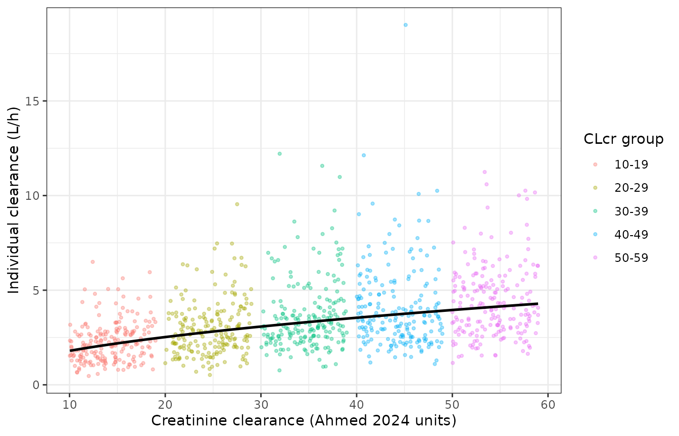
Replicates Figure 1 of Ahmed 2024: simulated individual vancomycin clearance versus creatinine clearance.
sim |>
  filter(!is.na(Cc)) |>
  group_by(grp, time) |>
  summarise(
    med = median(Cc), lo = quantile(Cc, 0.05), hi = quantile(Cc, 0.95),
    .groups = "drop"
  ) |>
  ggplot(aes(x = time, y = med, colour = grp, fill = grp)) +
  geom_ribbon(aes(ymin = lo, ymax = hi), alpha = 0.12, colour = NA) +
  geom_line(linewidth = 0.8) +
  labs(x = "Time (h)", y = "Vancomycin concentration (mg/L)",
       colour = "CLcr group", fill = "CLcr group") +
  theme_bw()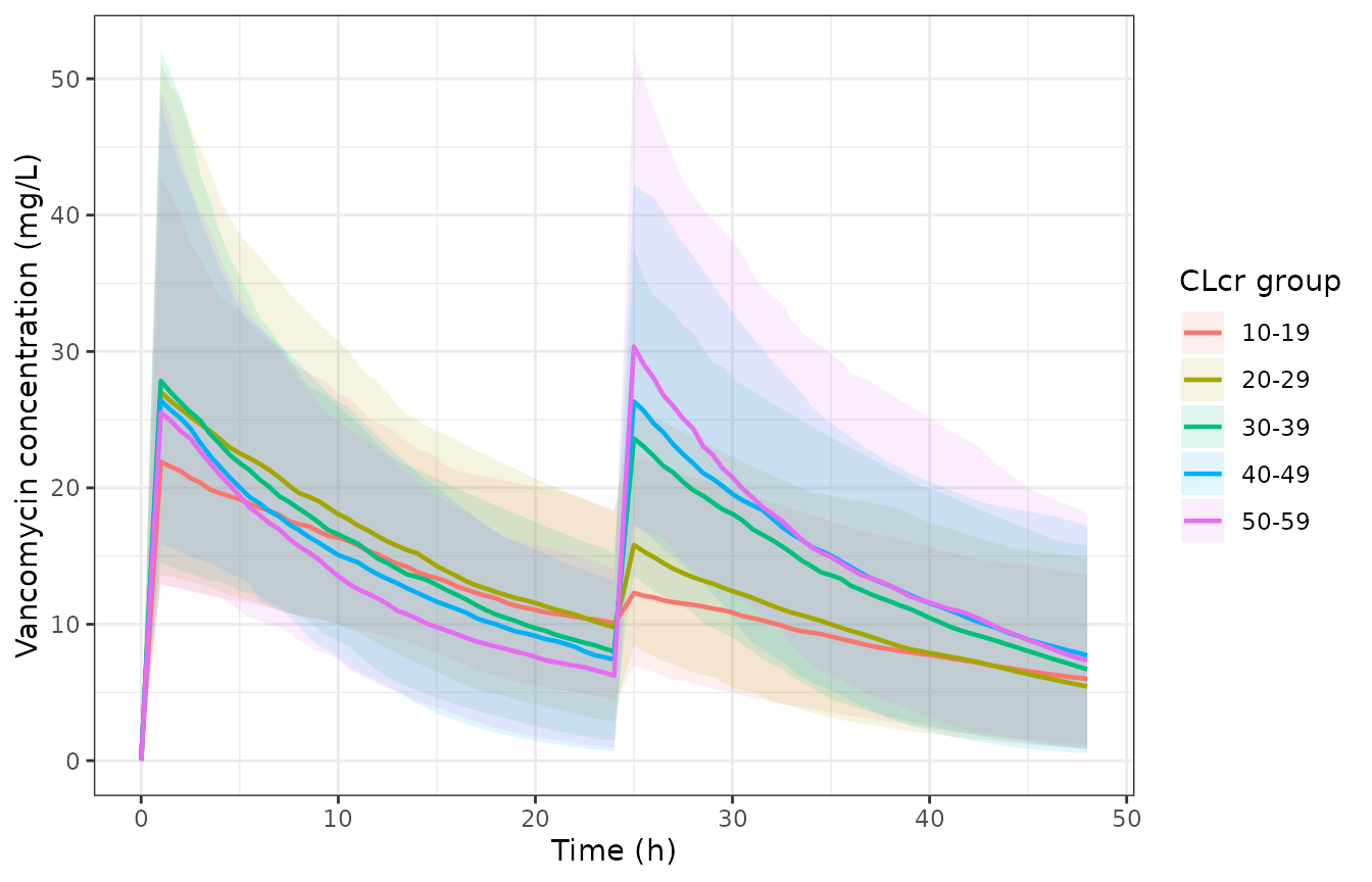
Median simulated vancomycin concentration-time profile by CLcr group, loading dose at 0 h and maintenance dose at 24 h.
Noncompartmental analysis (PKNCA)
AUC24-48 is the paper’s efficacy and safety endpoint, defined as the exposure on the second day of therapy with a target window of 400-600 mg.h/L (Methods, “Model-Based Dose Optimization”).
nca_conc <-
  sim |>
  filter(!is.na(Cc)) |>
  select(id, grp, time, Cc)

nca_dose <-
  doses |>
  select(id, grp, time, amt)

conc_obj <- PKNCA::PKNCAconc(nca_conc, Cc ~ time | grp + id)
dose_obj <- PKNCA::PKNCAdose(nca_dose, amt ~ time | grp + id)

intervals <- data.frame(
  start = 24, end = 48,
  auclast = TRUE, cmax = TRUE, cmin = TRUE
)

nca_res <- PKNCA::pk.nca(PKNCA::PKNCAdata(conc_obj, dose_obj, intervals = intervals))

nca_by_group <-
  as.data.frame(nca_res) |>
  group_by(grp, PPTESTCD) |>
  summarise(median = median(PPORRES), .groups = "drop") |>
  pivot_wider(names_from = PPTESTCD, values_from = median)

nca_by_group |>
  left_join(select(groups, grp, auc_pub), by = "grp") |>
  transmute(
    `CLcr group`               = grp,
    `Simulated AUC24-48`       = round(auclast, 1),
    `Published AUC24-48`       = auc_pub,
    `Difference (%)`           = round(100 * (auclast / auc_pub - 1), 1),
    `Simulated Cmax (mg/L)`    = round(cmax, 1),
    `Simulated Ctrough (mg/L)` = round(cmin, 1)
  ) |>
knitr::kable(caption = "PKNCA AUC24-48 (median across 200 subjects per group) against the AUC24-48 column of Ahmed 2024 Table 4.")| CLcr group | Simulated AUC24-48 | Published AUC24-48 | Difference (%) | Simulated Cmax (mg/L) | Simulated Ctrough (mg/L) |
|---|---|---|---|---|---|
| 10-19 | 222.3 | 455.62 | -51.2 | 12.6 | 6.4 |
| 20-29 | 232.8 | 489.89 | -52.5 | 14.6 | 5.5 |
| 30-39 | 307.5 | 503.46 | -38.9 | 22.1 | 7.0 |
| 40-49 | 333.9 | 492.39 | -32.2 | 25.5 | 6.2 |
| 50-59 | 370.6 | 491.78 | -24.6 | 30.9 | 5.9 |
The simulated exposures fall 25-55% below the published column. That gap is not a transcription slip on our side, and it is not attributable to any choice we made about dosing interval, infusion duration or volume of distribution – as the next section shows, the published values are unreachable.
The published AUC24-48 column exceeds what the model can produce
For a one-compartment model, mass balance over the window
[24, 48] gives
Write
.
The most the loading dose LD can leave at 24 h is
A(24) = LD \cdot r, and the least the window can end on is
A(48) = (A(24) + D) \cdot r, attained when the whole
maintenance dose D is given at the very start of the
window. Both extremes therefore give
The right-hand side is a downward parabola in r,
maximised at r* = (LD - D) / (2 LD) (or at
r* = 0 when D >= LD). Evaluating there
bounds AUC24-48for every possible volume of
distribution, every dosing interval within the window, and
every infusion duration – r is the only route by which any
of those enter. Substituting the paper’s own doses and its own Table 4
median clearances:
ceiling_tbl <-
  groups |>
  mutate(
    r_star  = pmax(0, (load - maint) / (2 * load)),
    ceiling = (load * r_star + maint) * (1 - r_star) / cl_pub
  ) |>
  transmute(
    `CLcr group`                = grp,
    `Loading dose (mg)`         = load,
    `Maintenance (mg/24 h)`     = maint,
    `Table 4 median CL (L/h)`   = cl_pub,
    `Maximum possible AUC24-48` = round(ceiling, 1),
    `Published AUC24-48`        = auc_pub,
    `Published exceeds max by`  = sprintf("%+.0f%%", 100 * (auc_pub / ceiling - 1))
  )
knitr::kable(ceiling_tbl,
caption = "A volume-free upper bound on AUC24-48. Every published value exceeds it.")| CLcr group | Loading dose (mg) | Maintenance (mg/24 h) | Table 4 median CL (L/h) | Maximum possible AUC24-48 | Published AUC24-48 | Published exceeds max by |
|---|---|---|---|---|---|---|
| 10-19 | 1500 | 200 | 2.22 | 217.0 | 455.62 | +110% |
| 20-29 | 1800 | 400 | 2.90 | 231.8 | 489.89 | +111% |
| 30-39 | 1800 | 1000 | 3.42 | 318.4 | 503.46 | +58% |
| 40-49 | 1800 | 1300 | 3.88 | 344.0 | 492.39 | +43% |
| 50-59 | 1800 | 1650 | 4.28 | 386.2 | 491.78 | +27% |
auc_ceiling <-
  with(groups, {
    r_star <- pmax(0, (load - maint) / (2 * load))
    (load * r_star + maint) * (1 - r_star) / cl_pub
  })
All five published AUC24-48 values exceed the model’s mathematical ceiling, by 27% in the least impaired group and by 110% in the most impaired. The AUC block of Tables 4 and 5 – and the probability-of-target-attainment columns derived from it – therefore cannot be reproduced from the published model and the published dosing regimen. The structural and variability parameters, which are what this package ships, are unaffected: they reproduce the clearance and volume columns of the same table.
Validation assertions
stopifnot(
  # Structural: typical-value clearance and volume reproduce the Table 4
  # medians. Deterministic (random effects zeroed), so a tight bound is
  # appropriate; the residual is the ~3-4% centering-constant offset.
  all(abs(typ$cl_pct) < 6),

  # V carries no covariate and no random effect in this run, so the typical
  # value is exactly V_pop = 65 L for all five groups. Asserted as an exact
  # identity rather than a tolerance: it is simultaneously the transcription
  # check on V_pop and the mechanical guard that zeroRe() + omega = NA really
  # did suppress the etas (a leaked eta makes these five values differ).
  max(abs(typ$vc - 65)) < 1e-8,
  all(abs(typ$vc_pct) < 3),

  # The mirror guard on the population solve: IIV must actually be present.
  dplyr::n_distinct(round(per_subject$vc, 8)) == nrow(per_subject),

  # Covariate direction and magnitude: clearance must rise monotonically with
  # CLcr, and by the published power across the simulated range.
  !is.unsorted(typ$cl),
  abs(typ$cl[5] / typ$cl[1] - (54.5 / 14.5)^0.49) < 0.01,

  # Stochastic cohort: gate the CENTRE, not the extremes. With 200 subjects
  # per arm the median carries a few percent of Monte Carlo noise on top of
  # the systematic offset.
  all(abs(sim_summary$cl_med / sim_summary$cl_pub - 1) < 0.15),
  all(abs(sim_summary$vc_med / sim_summary$vd_pub - 1) < 0.10),

  # Variability: the model's interquartile width matches the width Table 4
  # prints, while its 95% width does not - the basis for reading those
  # brackets as IQRs.
  all(abs(width_iqr / published_width - 1) < 0.10),
  all(width_95 / published_width > 2),

  # The published AUC24-48 column exceeds the volume-free ceiling in every
  # group, by at least 25%. Pure arithmetic on published numbers -- no
  # simulation, no random draw, so a tight bound is correct here.
  all(groups$auc_pub / auc_ceiling > 1.25),

  # Sanity: the simulation produced finite concentrations everywhere.
  all(is.finite(sim$Cc[!is.na(sim$Cc)])),
  nrow(per_subject) == 5L * n_per_group
)
Assumptions and deviations
-
Centering constant (12.7). The Methods define the
clearance covariate reference as
mean(CLcr); the paper never prints a mean for the covariate. The cohort median of 12.7 (Table 1) is used. Back-solving Ahmed 2024 Table 4 implies an effective reference near 11.8, consistent across all five CLcr groups, which leaves typical clearance about 3-4% low. That constant was deliberately not fitted to the validation target. -
Equation 5 versus the Methods equation. The paper
prints the clearance covariate model in two mutually inconsistent forms.
The centered Methods form (p. 83) is implemented; the uncentered
Equation 5 (p. 85, repeated in the Table 3 footnote) is treated as a
typesetting omission of the
/ mean(CLcr)denominator, on the evidence shown above that it overshoots the paper’s own simulated clearances roughly three-fold. -
CRCL is not a conventional creatinine clearance. It
is Bjornson’s
Rcrdivided by serum creatinine with the body-weight multiplier and the 14.4 unit divisor omitted, because weight was not recorded. Users must reproduce that calculation rather than substituting a Cockcroft-Gault value; see thecovariateData$CRCLnotes in the model file. - Table 4 / Table 5 bracket columns. Labelled “95% Interval”; they match the model’s interquartile range and not its 95% interval. Treated as IQRs throughout this vignette.
- Table 4 / Table 5 AUC24-48 and PTA columns are not reproducible. Every published AUC24-48 exceeds, by 27% to 110%, a volume-free mathematical ceiling derived from the paper’s own doses and its own median clearances – a bound that holds for every volume of distribution, dosing interval and infusion duration, so no modelling choice on our side can close it. Because the PTA columns are computed from that AUC distribution, they inherit the defect. This is a reporting error in the source, recorded here rather than worked around. The parameters this package ships are unaffected.
- Dosing regimen. The paper states the loading doses (Table 4 footnote a) and the total daily maintenance dose, but not the maintenance dosing interval or when maintenance begins. We give the loading dose at 0 h and the whole maintenance dose at 24 h. The AUC ceiling above holds for every alternative reading, so this choice does not drive the discrepancy.
- Infusion duration. 60 min for every dose, per Methods, “Dosing and Sample Collection”. The paper does not say whether the larger loading doses were infused more slowly.
- CLcr distribution within a group. Drawn uniformly across each group’s stated range, matching “1000 random values (according to the range of CLcr values for each group) were generated”. The paper does not state the distribution used.
- Cohort size. 200 subjects per CLcr group rather than the paper’s 1000 (x 20 replicates), to keep the vignette within its render budget. All assertions are made on medians and interquartile widths, which are stable at this size.
-
Covariates screened but not retained (age, serum
creatinine, serum albumin, blood urea nitrogen, sex) are recorded in
covariatesDataExcludedin the model file with their objective-function drops, not incovariateData. Sex has no published coefficient at all – the Discussion reports only that it dropped the OFV by 6.03 points before backward elimination removed it. - No errata. No correction, corrigendum or erratum to Ahmed 2024 was located.