Andrographolide (Songvut 2026)
Source:vignettes/articles/Songvut_2026_andrographolide.Rmd
Songvut_2026_andrographolide.RmdModel and source
mod <- readModelDb("Songvut_2026_andrographolide")
ui <- rxode2::rxode(mod)- Citation: Songvut P, Payoong P, Okada PA, Rittapai N, Suntararuks S, Akanimanee J, Rangkadilok N, Panomvana D, Puranajoti P, Satayavivad J. Exploratory pharmacokinetic-pharmacodynamic characterization and safety of standardized Andrographis paniculata aqueous extract capsules in patients with mild COVID-19. Front Pharmacol. 2026;17:1781740. doi:10.3389/fphar.2026.1781740. Model equation from Section 2.4 ‘Statistical analysis’; parameter values from Section 3.3.2 ‘PK/PD relationship’. The baseline term e0 is not printed anywhere in the paper and was recovered from Figure 5; see the ini() comment on le0 for the adjudication.
- Article: https://doi.org/10.3389/fphar.2026.1781740
- Supplement: https://www.frontiersin.org/articles/10.3389/fphar.2026.1781740/full#supplementary-material (Figures S1-S3 only: HPLC chromatograms, diterpenoid chemical structures, MS chromatograms. The supplement contains no model parameters.)
Description: Exploratory sigmoidal Emax exposure-response model relating andrographolide exposure to SARS-CoV-2 viral-load reduction in patients with mild COVID-19 treated with standardized Andrographis paniculata aqueous extract capsules (30 mg andrographolide every 8 h, 90 mg/day, for 5 consecutive days). The response is the log10 RdRp viral-load reduction between day 1 and day 5 and the driver is the day-5 andrographolide AUC(0-4 h), supplied as the AUC_ANDRO covariate column. This is a cross-sectional exposure-response layer only: there are no ODE states, no dosing events and no time dependence, so the pharmacokinetics are NOT part of this file (the source paper characterised them by non-compartmental analysis rather than by a population PK model). The model is a four-parameter sigmoid, baseline e0 plus a saturable increment: reduction = e0 + emax * AUC^hill / (auc50^hill + AUC^hill). The nonzero baseline captures spontaneous viral clearance in this uncontrolled single-arm study and is figure-derived, not printed (see the ini() comment on le0 and the vignette Errata). Fit by unweighted nonlinear regression in GraphPad Prism to n = 12 patients at a single dose level, so the parameters are hypothesis-generating rather than confirmatory: the paper reports r2 = 0.4 and could not estimate confidence intervals for any parameter. There is no between-subject variability (the source fitted a single typical-value curve to the pooled cohort).
What this paper contributes, and what it does not
Songvut 2026 is an open-label, single-centre, single-arm pharmacokinetic / pharmacodynamic and safety study of standardized Andrographis paniculata aqueous extract capsules in 12 Thai adults with mild COVID-19. It reports two distinct analyses, and only one of them is a fitted model:
-
The pharmacokinetics are non-compartmental only.
Table 2 reports Cmax, Tmax, AUC(0-4 h), AUC(0-inf), MRT, Vd/F, Cl/F and
half-life for each of the four major diterpenoids, computed in PK
Solutions 2.0 by the linear trapezoidal rule (paper Section 2.3.6).
Cl/F,Vd/Fandt1/2there are NCA-derived summary statistics, not a fitted structural model. There is no population PK model in the paper, and therefore none in this package: nothing inSongvut_2026_andrographolideproduces a concentration-time profile. - The exposure-response relationship is a fitted model, and it is what this package reproduces: an exploratory sigmoidal Emax curve relating each patient’s day-5 andrographolide AUC(0-4 h) to their log10 RdRp viral-load reduction between day 1 and day 5, fitted by unweighted nonlinear regression in GraphPad Prism 9.3.0 (paper Sections 2.4 and 3.3.2, Figure 5).
Because there is no PK layer, this vignette has no PKNCA section:
there is no concentration-time profile to integrate and no simulated NCA
parameter to compare against Table 2. The validation instead follows the
package’s pattern for mechanistic and algebraic models – closed-form
agreement, anchor reproduction, monotonicity and boundedness, and a
goodness-of-fit round trip against the paper’s own reported
r2. The published NCA table is transcribed below for
context, clearly marked as reference-only.
The paper is emphatic, and this vignette repeats it, that the exposure-response analysis is exploratory and hypothesis-generating, not confirmatory. There was no placebo arm, so the observed viral-load decline overlaps the expected window of natural clearance in vaccinated patients with mild COVID-19 and cannot be attributed to the extract. With n = 12 at a single dose level and a narrow exposure range, the paper could not estimate a confidence interval for any parameter.
Population
Twelve adults (10 female, 2 male; 83.33% female) of Thai nationality, aged 18-60 years by inclusion criterion with a mean age of 34.08 +/- 9.29 years and a mean body mass index of 21.07 +/- 2.19 kg/m^2, all with RT-PCR-confirmed SARS-CoV-2 infection within 72 h of symptom onset and classified as mild COVID-19 under the WHO 2020 clinical-management guidance – symptomatic without viral pneumonia or hypoxia, resting SpO2 at least 95%, normal chest radiograph (paper Tables 3-5 and Section 2.3.1). All were vaccinated, with the most recent dose more than one year before enrollment, and none had significant comorbidities. Body weight is not reported; only BMI is, so no weight-based scaling is possible or needed.
Each participant received capsules equivalent to a labelled 30 mg of andrographolide (three capsules of 10 mg labelled content; measured content 10.28 +/- 0.03 mg per capsule, paper Table 1) every 8 h for 5 consecutive days, i.e. 90 mg/day, alongside as-needed symptomatic standard of care. Intensive 0-4 h plasma sampling was performed after the first dose on day 1 and again after the morning dose on day 5. All 12 completed the protocol with 100% compliance, no dropouts and no protocol deviations, so all 12 contribute to the exposure-response fit.
The same information is available programmatically:
str(readModelDb("Songvut_2026_andrographolide")()$population)
#> List of 13
#>  $ species       : chr "human"
#>  $ n_subjects    : int 12
#>  $ n_studies     : int 1
#>  $ age_range     : chr "18-60 years (inclusion criterion); mean 34.08 +/- 9.29 years, two participants classified as middle-aged adults"
#>  $ age_median    : chr "(not reported in Songvut 2026; mean 34.08 years)"
#>  $ weight_range  : chr "(not reported in Songvut 2026; body mass index 21.07 +/- 2.19 kg/m^2, and obesity with BMI > 35 kg/m^2 was an e"| __truncated__
#>  $ weight_median : chr NA
#>  $ sex_female_pct: num 83.3
#>  $ race_ethnicity: Named num 100
#>   ..- attr(*, "names")= chr "Asian"
#>  $ disease_state : chr "Mild COVID-19 by the WHO 2020 clinical-management classification: RT-PCR-confirmed SARS-CoV-2 infection within "| __truncated__
#>  $ dose_range    : chr "Single dose level. Standardized A. paniculata aqueous extract capsules equivalent to a labelled 30 mg of androg"| __truncated__
#>  $ regions       : chr "Thailand (single centre: acute respiratory infection clinic, Chulabhorn Hospital, Chulabhorn Royal Academy, Bangkok)"
#>  $ notes         : chr "Baseline demographics and clinical laboratory values in paper Table 5; per-subject viral loads and log10 reduct"| __truncated__
Source trace
Per-parameter origins are recorded as in-file comments beside each
ini() entry in
inst/modeldb/specificDrugs/Songvut_2026_andrographolide.R.
Collected here:
| Equation / parameter | Value | Source location |
|---|---|---|
| Sigmoidal Emax equation | Effect = Emax * AUC^gamma / (EAUC50^gamma + AUC^gamma) |
Section 2.4 “Statistical analysis”, displayed equation |
Baseline term e0 added to the printed equation |
1.81 | Not printed. Recovered from Figure 5; see “The printed equation versus Figure 5” below |
lemax = log(2.24) |
2.24 -log10 copies/uL | Section 3.3.2: “Emax = 2.24 log10 copies/mL” |
lauc50 = log(29.80) |
29.80 ug*h/L | Section 3.3.2: “EAUC50 = 29.80 ug h/L”; corroborated in Section 4.3 |
lhill = log(8) |
8 (unitless) | Section 3.3.2: “The Hill coefficient was estimated to be approximately 8 and approached the upper boundary of the constrained parameter range” |
addSd = 1.245 |
1.245 -log10 copies/uL |
Derived, not printed: from r2 = 0.4
(Section 3.3.2) and the 12 log10 reductions in Table 3, using ordinary
least squares (Section 2.4: “Nonlinear regression was performed without
weighting”) |
| Reported goodness of fit |
r2 = 0.4 |
Section 3.3.2 |
AUC_ANDRO covariate |
day-5 AUC(0-4 h), mean 30.12 +/- 15.83 ug*h/L | Table 2, andrographolide (AP1) block; Figure 5 x-axis |
| Per-subject response values | 12 log10 reductions, 0.20 to 5.10 | Table 3, “Log10 reduction (between day 1 and 5)” column |
| No between-subject variability | n/a | Section 2.4 – a single curve fitted by nonlinear regression to the pooled cohort; no hierarchical model |
| No covariate effects | n/a | The paper screened no covariates on the exposure-response model |
The printed equation versus Figure 5
This is the one place where the packaged model deliberately departs from the paper’s printed equation, so the reasoning is set out in full.
The equation printed in Section 2.4 is a three-parameter sigmoid with no baseline term:
Effect = Emax * AUC^gamma / (EAUC50^gamma + AUC^gamma)Under that form, with the printed Emax = 2.24,
EAUC50 = 29.80 and gamma = 8, the curve would
run from 0 at zero exposure to 2.24 at saturation, and the half-maximal
point would sit at y = 1.12. Figure 5 shows something else: a lower
asymptote near 1.85, a plateau near 4.05 carrying the “Emax” annotation,
and the dashed EAUC50 guide line drawn at y near 3.0.
Three independent pieces of the paper’s own evidence adjudicate this, and all three point the same way – the fitted curve carries a nonzero baseline:
-
The plateau.
e0 + emax= 1.81 + 2.24 = 4.05 reproduces the figure’s plateau, the point the figure labels “Emax”. -
The guide line.
e0 + emax/2= 2.93 reproduces where the dashedEAUC50line is drawn (y near 3.0), rather than the 1.12 the printed form requires. -
The reported goodness of fit. Scored against the
paper’s own 12 response values (Table 3) and the digitised Figure 5
exposures, the printed three-parameter form gives
r2= -0.90 – worse than predicting the mean – while the four-parameter form givesr2= +0.37, which is the paper’s reported 0.4. The printed form cannot reproduce the paper’s own stated fit.
The most likely explanation is typesetting: GraphPad Prism’s standard
sigmoidal dose-response models are parameterised with
Bottom and Top, so the reported “Emax = 2.24”
is the Top - Bottom increment rather than
the absolute plateau, and the displayed equation dropped the
Bottom term.
The packaged model therefore encodes the four-parameter form
reduction = e0 + emax * AUC^hill / (auc50^hill + AUC^hill)with e0 = 1.81 recovered from Figure 5. This resolution
was ratified by the maintainers (see Assumptions and deviations). The
e0 term is not a fudge factor: in an uncontrolled
single-arm study it is exactly the quantity the design cannot separate
from drug effect – spontaneous viral clearance – which is why the
paper’s own Discussion stresses that the decline cannot be attributed to
the extract.
Digitised Figure 5 data
The 12 response values are printed exactly in Table 3. The 12 matching exposures are not tabulated per subject anywhere in the paper, only plotted, so they were digitised from Figure 5.
fig5 <- tibble::tibble(
  # x: per-subject day-5 AUC(0-4 h), digitised from Figure 5 (ug*h/L).
  AUC_ANDRO = c(7.5, 11.5, 16.0, 14.0, 23.0, 30.0, 36.0, 39.5, 40.0, 46.0, 43.5, 57.0),
  # y: per-subject log10 viral-load reduction, EXACT from paper Table 3.
  observed  = c(2.12, 4.83, 1.31, 0.40, 0.20, 3.09, 4.01, 5.10, 4.31, 4.05, 2.31, 3.84)
)
stopifnot(nrow(fig5) == 12L)
The digitisation is validated independently of anything it is later used for: the paper reports the cohort’s day-5 AUC(0-4 h) as 30.12 +/- 15.83 ug*h/L in Table 2, a number that played no part in reading the figure.
auc_mean <- mean(fig5$AUC_ANDRO)
auc_sd <- sd(fig5$AUC_ANDRO)
c(mean = auc_mean, sd = auc_sd)
#>     mean       sd
#> 30.33333 15.78741

# Table 2, andrographolide (AP1), 90 mg/day column: 30.12 +/- 15.83 ug*h/L.
stopifnot(
  abs(auc_mean - 30.12) / 30.12 < 0.02,
  abs(auc_sd - 15.83) / 15.83 < 0.05
)

# The response values must be Table 3's, not a re-reading of the figure: their
# arithmetic mean is the paper's reported day-5 reduction of 2.96 log10.
stopifnot(abs(mean(fig5$observed) - 2.96) < 0.01)
Both the centre and the spread of the digitised exposures land on the independently published values, which is a strong check that the x-axis was read correctly. Note the caveats: Table 3 lists two nearly identical responses (4.01 and 4.05) whose assignment between the x = 36 and x = 46 points cannot be resolved from the figure, an ambiguity of 0.04 log10 that moves nothing; and individual digitised exposures carry roughly +/- 1 ug*h/L of reading error.
Simulation
The model is algebraic and cross-sectional – no ODE states, no dosing
events, no time dependence – so an event table is observation rows only,
each carrying that subject’s AUC_ANDRO.
events_cohort <- fig5 |>
  mutate(id = row_number(), time = 0, evid = 0L) |>
  select(id, time, evid, AUC_ANDRO)

# Join on `id`, not on AUC_ANDRO: joining on a floating-point covariate that
# has round-tripped through the solver is a needless footgun.
sim_cohort <- solve_er(ui, events_cohort) |>
  select(id, predicted = viral_loadReduction) |>
  left_join(mutate(fig5, id = row_number()), by = "id")

stopifnot(nrow(sim_cohort) == 12L, !anyNA(sim_cohort$predicted))
A dense exposure grid gives the fitted curve. It stays inside the 200-per-arm cohort cap.
grid_auc <- seq(0, 60, length.out = 121)
stopifnot(length(grid_auc) <= 200L)

curve <- solve_er(
  ui,
  data.frame(id = seq_along(grid_auc), time = 0, evid = 0L, AUC_ANDRO = grid_auc)
) |>
  select(AUC_ANDRO, predicted = viral_loadReduction)
Validation
Gate 1 – rxode2 solve equals the closed form exactly
Both sides use the same parameter draw, so the only difference is numerical. A tight bound is correct here.
pars <- ui$theta
e0 <- exp(pars[["le0"]])
emax <- exp(pars[["lemax"]])
auc50 <- exp(pars[["lauc50"]])
hill <- exp(pars[["lhill"]])
c(e0 = e0, emax = emax, auc50 = auc50, hill = hill)
#>    e0  emax auc50  hill
#>  1.81  2.24 29.80  8.00

analytic <- er_closed_form(curve$AUC_ANDRO, e0, emax, auc50, hill)
max_abs_err <- max(abs(curve$predicted - analytic))
max_abs_err
#> [1] 0

stopifnot(length(analytic) == 121L, max_abs_err < 1e-8)
Gate 2 – the three Figure 5 anchors
The lower asymptote, the dashed EAUC50 guide line and
the labelled plateau are three separately readable features of Figure 5.
All three must fall out of the encoded parameters.
anchors <- solve_er(
  ui,
  data.frame(
    id = 1:3, time = 0, evid = 0L,
    AUC_ANDRO = c(0, auc50, 1e6)  # zero exposure, half-maximal, saturating
  )
) |>
  transmute(
    anchor = c("lower asymptote (AUC = 0)", "at EAUC50", "plateau (saturating)"),
    predicted = viral_loadReduction,
    figure5 = c(1.81, 2.93, 4.05)
  )

anchors |>
  rename("Figure 5 feature" = anchor,
         "Model" = predicted,
         "Read from Figure 5" = figure5) |>
knitr::kable(digits = 4, caption = "Gate 2: the encoded curve reproduces all three readable features of Figure 5.")| Figure 5 feature | Model | Read from Figure 5 |
|---|---|---|
| lower asymptote (AUC = 0) | 1.81 | 1.81 |
| at EAUC50 | 2.93 | 2.93 |
| plateau (saturating) | 4.05 | 4.05 |
Gate 3 – monotone and bounded over the observed exposure range
A sigmoidal Emax curve with a positive Hill coefficient must increase
monotonically and stay within [e0, e0 + emax]. This catches
a sign error or a mistyped exponent that the anchor gate alone would
not.
stopifnot(
  all(diff(curve$predicted) > 0),
  all(curve$predicted >= e0 - 1e-9),
  all(curve$predicted <= e0 + emax + 1e-9),
  # Hill = 8 makes the transition sharp: essentially all of the increment is
  # spent between half and double the EAUC50.
  er_closed_form(auc50 / 2, e0, emax, auc50, hill) < e0 + 0.01 * emax,
  er_closed_form(auc50 * 2, e0, emax, auc50, hill) > e0 + 0.99 * emax
)
Gate 4 – the encoded model reproduces the paper’s reported r2
The paper reports r2 = 0.4 (Section 3.3.2), to one
significant figure. The encoded model, scored against the paper’s own 12
response values, must land there – and the printed three-parameter
alternative must not.
sst <- sum((sim_cohort$observed - mean(sim_cohort$observed))^2)
r2_of <- function(pred) 1 - sum((sim_cohort$observed - pred)^2) / sst

r2_encoded <- r2_of(sim_cohort$predicted)
r2_printed <- r2_of(er_closed_form(sim_cohort$AUC_ANDRO, 0, emax, auc50, hill))

tibble::tibble(
  form = c("Encoded: 4-parameter, e0 = 1.81",
           "Printed Section 2.4: 3-parameter, no baseline"),
  r2 = c(r2_encoded, r2_printed)
) |>
  rename("Model form" = form, "r2 vs the paper's 12 responses" = r2) |>
knitr::kable(digits = 3, caption = "Gate 4: only the encoded four-parameter form reproduces the paper's reported r2 of 0.4.")| Model form | r2 vs the paper’s 12 responses |
|---|---|
| Encoded: 4-parameter, e0 = 1.81 | 0.367 |
| Printed Section 2.4: 3-parameter, no baseline | -0.899 |
Gate 5 – the encoded residual SD round-trips
addSd was derived from the reported r2 =
0.4 and Table 3’s responses, so this gate is not circular: it asks
whether the SD implied by the encoded model’s actual residuals
agrees with the value derived from the reported fit. A
structural transcription error would separate the two.
rmse_actual <- sqrt(mean((sim_cohort$observed - sim_cohort$predicted)^2))
addSd_encoded <- pars[["addSd"]]
c(rmse_actual = rmse_actual, addSd_encoded = addSd_encoded,
  pct_diff = 100 * (rmse_actual - addSd_encoded) / addSd_encoded)
#>   rmse_actual addSd_encoded      pct_diff
#>      1.278408      1.245000      2.683383

stopifnot(abs(rmse_actual - addSd_encoded) / addSd_encoded < 0.05)
The residual error is large relative to the effect it sits on – an SD
of about 1.25 log10 against a total modelled range of 2.24 log10. That
is the honest picture of an r2 = 0.4 fit to 12 patients,
and it is why the paper declines to treat these parameters as
confirmatory.
The stochastic layer is exercised once to confirm the error model is wired up and that the residual band brackets the observations.
set.seed(20260901)
rxode2::rxSetSeed(20260901)

rep_events <- tidyr::expand_grid(replicate = 1:50, fig5) |>
  mutate(id = row_number(), time = 0, evid = 0L) |>
  select(id, time, evid, AUC_ANDRO)

rep_sim <- solve_er(ui, rep_events)
sd_sim <- sd(rep_sim$sim - rep_sim$viral_loadReduction)
c(addSd_encoded = addSd_encoded, sd_of_simulated_residuals = sd_sim)
#>             addSd_encoded sd_of_simulated_residuals
#>                  1.245000                  1.291494

stopifnot(
  nrow(rep_sim) == 600L,
  # 600 draws recover the encoded SD to well within Monte Carlo error.
  abs(sd_sim - addSd_encoded) / addSd_encoded < 0.10
)
Gate 6 – the paper’s “AUC approached EAUC50” claim
Sections 3.3.2 and 4.3 both state that the day-5 mean AUC(0-4 h) of
30.12 ugh/L approached the estimated EAUC50 of 29.80
ugh/L, i.e. that the regimen sat near the steep middle of the
curve. That is a checkable claim about the encoded model, not just about
two numbers.
at_cohort_mean <- er_closed_form(30.12, e0, emax, auc50, hill)
half_maximal <- e0 + emax / 2
frac_of_increment <- (at_cohort_mean - e0) / emax
c(exposure_excess_over_auc50 = 30.12 / auc50 - 1,
  at_cohort_mean = at_cohort_mean, half_maximal = half_maximal,
  fraction_of_max_increment = frac_of_increment)
#> exposure_excess_over_auc50             at_cohort_mean
#>                 0.01073826                 2.97782183
#>               half_maximal  fraction_of_max_increment
#>                 2.93000000                 0.52134903

stopifnot(
  # The cohort mean exposure sits 1.07% above auc50.
  abs(30.12 / auc50 - 1) < 0.02,
  # Which puts the response within 2.2 percentage points of half-maximal.
  abs(frac_of_increment - 0.5) < 0.025,
  abs(at_cohort_mean - half_maximal) / half_maximal < 0.02
)
Note how the steep Hill coefficient amplifies: the cohort mean
exposure is only 1.07% above auc50, but that becomes a 2.1%
excess in the effect increment. With hill = 8 the curve is
so sharp near auc50 that small exposure differences
translate into disproportionate predicted-response differences – another
reason to treat the fitted steepness as poorly identified rather than
mechanistic.
Gate 7 – dimensional analysis
AUC_ANDRO and auc50 must share units so the
sigmoid is dimensionless, and e0, emax and
addSd must all be on the log10-reduction scale. Scaling
both exposure terms by any common factor must leave the prediction
unchanged.
str(ui$units)
#> List of 3
#>  $ time         : chr "day"
#>  $ dosing       : chr "(none; andrographolide exposure enters as the AUC_ANDRO covariate, not as a dose record)"
#>  $ concentration: chr "(log10 RdRp viral-load reduction between day 1 and day 5, -log10 copies/uL; the AUC_ANDRO exposure covariate is in ug*h/L)"

# Exposure enters only as AUC/auc50 ratios, so a common rescaling is a no-op.
scaled <- er_closed_form(fig5$AUC_ANDRO * 1000, e0, emax, auc50 * 1000, hill)
stopifnot(max(abs(scaled - sim_cohort$predicted)) < 1e-9)
Replicate Figure 5
# Replicates Figure 5 of Songvut 2026: exploratory exposure-effect relationship
# between day-5 andrographolide AUC(0-4 h) and log10 RdRp viral-load reduction.
ggplot(curve, aes(AUC_ANDRO, predicted)) +
  geom_hline(yintercept = e0 + emax, linetype = "dotted", colour = "grey40") +
  geom_segment(
    aes(x = 0, xend = auc50, y = half_maximal, yend = half_maximal),
    linetype = "dashed", colour = "grey40"
  ) +
  geom_segment(
    aes(x = auc50, xend = auc50, y = 0, yend = half_maximal),
    linetype = "dashed", colour = "grey40"
  ) +
  geom_line(linewidth = 1.2, colour = "#2C7FB8") +
  geom_point(data = fig5, aes(AUC_ANDRO, observed), shape = 4, size = 2.5) +
  annotate("text", x = 58, y = e0 + emax + 0.18, label = "Emax",
           colour = "#2C7FB8", hjust = 1) +
  annotate("text", x = auc50, y = -0.25, label = "EAUC50", size = 3) +
  coord_cartesian(xlim = c(0, 60), ylim = c(0, 6), clip = "off") +
  labs(
    x = "AUC(0-4 h, day 5) (ug*h/L)",
    y = "Decrease in log10 viral load\n(-log10 copies/uL)",
    title = "Figure 5 - exposure-effect relationship",
    caption = paste(
      "Replicates Figure 5 of Songvut 2026. Crosses are the 12 patients:",
      "responses exact from Table 3, exposures digitised from the figure."
    )
  ) +
  theme_bw()
#> Warning in geom_segment(aes(x = 0, xend = auc50, y = half_maximal, yend = half_maximal), : All aesthetics have length 1, but the data has 121 rows.
#> ℹ Please consider using `annotate()` or provide this layer with data containing
#>   a single row.
#> Warning in geom_segment(aes(x = auc50, xend = auc50, y = 0, yend = half_maximal), : All aesthetics have length 1, but the data has 121 rows.
#> ℹ Please consider using `annotate()` or provide this layer with data containing
#>   a single row.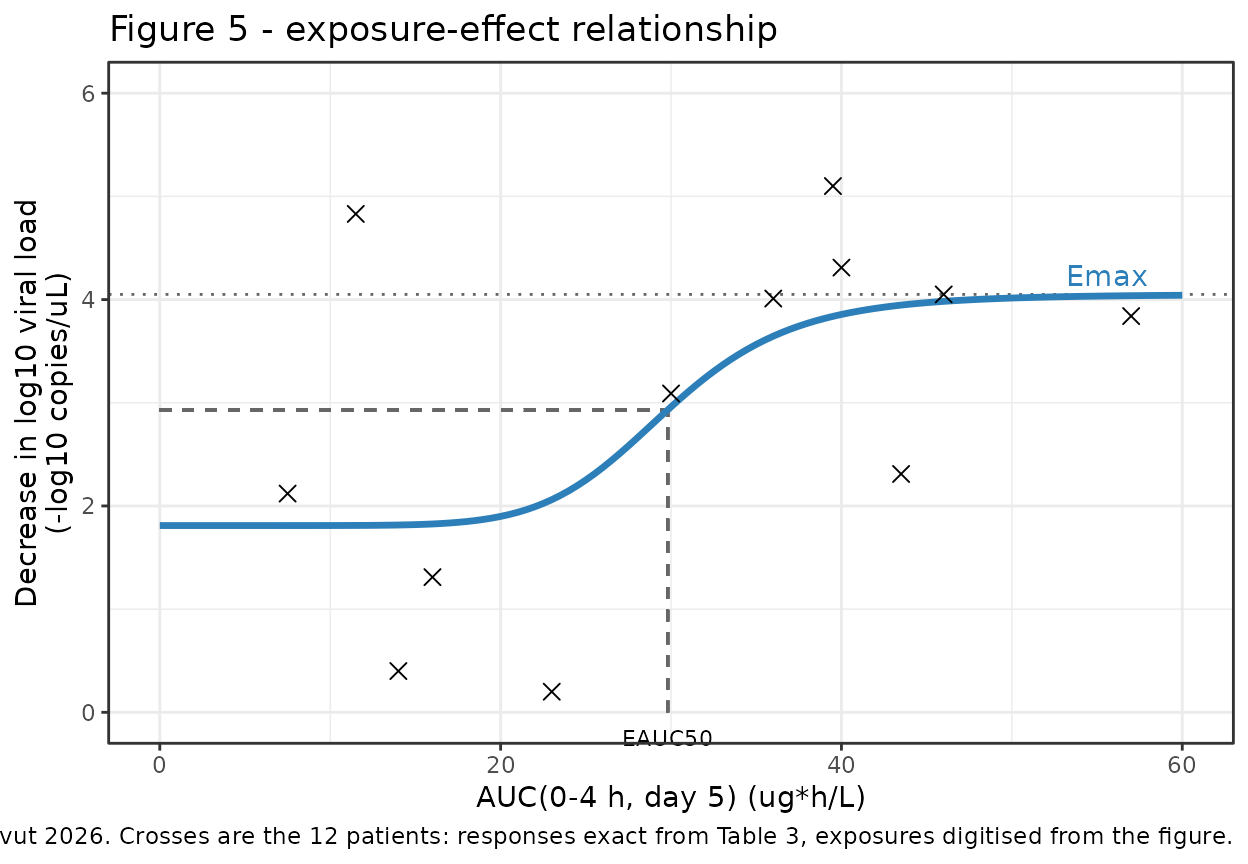
The reproduced panel matches the published figure feature for
feature: the nonzero lower asymptote, the plateau annotated
Emax, and the dashed guide lines meeting the curve at
EAUC50 on the x-axis and near y = 3 on the y-axis.
Observed versus predicted
sim_cohort |>
  arrange(AUC_ANDRO) |>
  mutate(residual = observed - predicted) |>
  select(AUC_ANDRO, observed, predicted, residual) |>
  rename(
    "AUC(0-4 h, day 5) (ug*h/L)" = AUC_ANDRO,
    "Observed reduction (log10)" = observed,
    "Model-predicted reduction (log10)" = predicted,
    "Residual (log10)" = residual
  ) |>
knitr::kable(digits = 3, caption = "Per-patient observed versus predicted log10 viral-load reduction. Observed values are exact from Table 3; exposures are digitised from Figure 5.")| AUC(0-4 h, day 5) (ug*h/L) | Observed reduction (log10) | Model-predicted reduction (log10) | Residual (log10) |
|---|---|---|---|
| 7.5 | 2.12 | 1.810 | 0.310 |
| 11.5 | 4.83 | 1.811 | 3.019 |
| 14.0 | 0.40 | 1.815 | -1.415 |
| 16.0 | 1.31 | 1.825 | -0.515 |
| 23.0 | 0.20 | 2.061 | -1.861 |
| 30.0 | 3.09 | 2.960 | 0.130 |
| 36.0 | 4.01 | 3.645 | 0.365 |
| 39.5 | 5.10 | 3.837 | 1.263 |
| 40.0 | 4.31 | 3.856 | 0.454 |
| 43.5 | 2.31 | 3.946 | -1.636 |
| 46.0 | 4.05 | 3.983 | 0.067 |
| 57.0 | 3.84 | 4.038 | -0.198 |
The two largest residuals are the patient at 11.5 ugh/L who cleared 4.83 log10 and the patient at 23.0 ugh/L who cleared only 0.20 log10 – both at the low end of the exposure range. This is the pattern the paper itself flags in Section 4.3: “greater variability in viral load reduction was observed at lower AUC levels, indicating limitations of the model in lower exposure range.”
Published non-compartmental parameters (reference only)
Transcribed from Table 2, andrographolide (AP1) block. These
are not gated against anything: the paper reports no PK model,
so this package cannot simulate a concentration-time profile to compare
them with. They are here so a downstream user assembling a PK layer for
AUC_ANDRO has the published targets in one place.
tibble::tribble(
  ~parameter,             ~single_dose,     ~multiple_dose,
  "Cmax (ug/L)",          "18.63 +/- 11.81", "17.82 +/- 10.56",
  "Tmax (h)",             "0.75 [0.31]",     "0.75 [0.5]",
  "AUC(0-4 h) (ug*h/L)",  "28.54 +/- 8.72",  "30.12 +/- 15.83",
  "AUC(0-inf) (ug*h/L)",  "32.81 +/- 8.91",  "not reported",
  "MRT (h)",              "2.15 +/- 0.69",   "4.19 +/- 3.88",
  "Vd/F (L/kg)",          "27.47 +/- 13.55", "41.02 +/- 32.22",
  "Cl/F (L/h/kg)",        "14.48 +/- 3.66",  "15.05 +/- 11.67",
  "Half-life (h)",        "1.21 [0.19]",     "1.48 [1.99]"
) |>
  rename(
    "NCA parameter" = parameter,
    "Single dose, 30 mg (n = 12)" = single_dose,
    "Multiple dose, 90 mg/day (n = 12)" = multiple_dose
  ) |>
knitr::kable(caption = "Songvut 2026 Table 2, andrographolide (AP1). Mean +/- SD, except Tmax and half-life as median [IQR]. Reference only - not reproducible from this package, which contains no PK model.")| NCA parameter | Single dose, 30 mg (n = 12) | Multiple dose, 90 mg/day (n = 12) |
|---|---|---|
| Cmax (ug/L) | 18.63 +/- 11.81 | 17.82 +/- 10.56 |
| Tmax (h) | 0.75 [0.31] | 0.75 [0.5] |
| AUC(0-4 h) (ug*h/L) | 28.54 +/- 8.72 | 30.12 +/- 15.83 |
| AUC(0-inf) (ug*h/L) | 32.81 +/- 8.91 | not reported |
| MRT (h) | 2.15 +/- 0.69 | 4.19 +/- 3.88 |
| Vd/F (L/kg) | 27.47 +/- 13.55 | 41.02 +/- 32.22 |
| Cl/F (L/h/kg) | 14.48 +/- 3.66 | 15.05 +/- 11.67 |
| Half-life (h) | 1.21 [0.19] | 1.48 [1.99] |
Assumptions and deviations
-
The encoded model departs from the printed equation by
adding a baseline term
e0. The paper’s Section 2.4 prints a three-parameter sigmoid with no baseline. The packaged model is the four-parameter forme0 + emax * AUC^hill / (auc50^hill + AUC^hill). This was escalated to the maintainers rather than decided silently, because recovering a value from a figure to fill a reporting gap is routine while using one to override a printed structural claim is not, and this act does both. It was ratified on 2026-08-31 on the evidence set out in “The printed equation versus Figure 5” above: the printed form cannot reproduce the paper’s own reportedr2, and the four-parameter form additionally reproduces two further independent Figure 5 features (plateau, guide line) that the printed form cannot explain. Gate 4 above is the load-bearing check. -
Non-paper-derived parameter value:
e0= 1.81 is not printed anywhere in the paper. It was recovered as the least-squares baseline withemax,auc50andhillheld at their printed values, fitted to Table 3’s responses against the digitised Figure 5 exposures (recovered 1.809), and it is also the value read directly off the Figure 5 lower asymptote. Treat it as carrying the uncertainty of a figure reading, roughly +/- 0.05 log10. -
Derived parameter value:
addSd= 1.245 is not printed either, but unlikee0it needs no figure: it follows from two printed quantities, since unweighted nonlinear regression (Section 2.4) means ordinary least squares and thereforer2 = 1 - SSE/SST, withSSTcomputable exactly from Table 3’s 12 responses. Thendenominator matches nlmixr2’s maximum-likelihood SD parameterisation; the degrees-of-freedom-corrected alternative with four estimated parameters would be 1.52. Becauser2is printed to one significant figure, this SD is only determined to about +/- 0.05. - Per-subject exposures are digitised from Figure 5, since the paper tabulates the responses (Table 3) but not the matching per-subject AUC values. The digitisation is validated against Table 2’s independently reported 30.12 +/- 15.83 ugh/L (Gate above). Individual values carry roughly +/- 1 ugh/L of reading error, and the assignment of Table 3’s 4.01 versus 4.05 between the two right-hand points cannot be resolved from the figure – a 0.04 log10 ambiguity that changes no conclusion. The digitised exposures are used only for validation in this vignette; no packaged parameter depends on an individual digitised value.
-
The Hill coefficient is at a boundary. The paper
states it “was estimated to be approximately 8 and approached the upper
boundary of the constrained parameter range”, but does not report the
bound. It is encoded as 8 and is not wrapped in
fixed(), because it was estimated rather than held; but the steepness it implies is poorly identified and should not be read as a mechanistic finding. Gate 3 shows how sharp it makes the transition: withhill= 8, essentially the whole effect increment is spent between half and double theEAUC50. - No between-subject variability and no covariate effects are encoded, because the source has none. The paper fitted a single typical-value curve to the pooled 12-patient cohort by nonlinear regression, with no hierarchical structure, and screened no covariates on the exposure-response model. No variance components were invented to fill the gap.
-
Units of
Emax. Section 3.3.2 givesEmaxin “log10 copies/mL” while Table 3 tabulates viral loads and log10 reductions in copies/uL. A log10 ratio is dimensionless, so the value is unaffected; the model file and this vignette use the Table 3 convention (-log10 copies/uL). -
Convention-lint deviation: the observation variable is
viral_loadReduction.checkModelConventions()warns that this is not a registered single-output canonical. The registeredviral_loadname is not appropriate – the endpoint is a change from baseline between two days, not a viral load, and the model has no baseline load from which one could be reconstructed (per-subject baselines in Table 3 span 541 to 4.4e6 copies/uL). The warning is accepted rather than papered over, following the same shape as other change-from-baseline single-output models already in the library (Morganroth_2015_moxifloxacin.RwithDDQTcF,Gong_2023_pemigatinib_creatinine.RwithcreatPctChange). Promoting aviral_loadReductioncanonical is left to the maintainers. -
No PK layer, and therefore no PKNCA validation. See
“What this paper contributes, and what it does not”. Downstream users
must supply
AUC_ANDROfrom observed concentrations or from an external andrographolide PK model; none exists for this formulation in the published literature. - No erratum applies. No correction notice was found for this article.
- The supplement contains no model parameters (Figures S1-S3 only), so nothing in the model file derives from it.
- Exploratory status. Every parameter here comes from an uncontrolled, single-arm, single-dose-level fit to 12 patients for which the paper could not estimate confidence intervals. The model reproduces what was published; it does not establish that andrographolide exposure causes viral-load reduction, and the paper explicitly declines that inference.