Docetaxel (Puisset 2007)
Source:vignettes/articles/Puisset_2007_docetaxel.Rmd
Puisset_2007_docetaxel.RmdModel and source
- Citation: Puisset F, Alexandre J, Treluyer J-M, Raoul V, Roche H, Goldwasser F, Chatelut E. (2007). Clinical pharmacodynamic factors in docetaxel toxicity. British Journal of Cancer 97(3):290-296. doi:10.1038/sj.bjc.6603872. PD structure follows Friberg LE et al. (2002) J Clin Oncol 20(24):4713-4721 (see modellib(‘Friberg_2002_paclitaxel’) for the leukocyte sibling). Upstream docetaxel PK was supplied via Bayesian individual posthoc profiles from Baille P et al. (1997) Clin Cancer Res 3:1535-1538 (built on the Bruno R et al. (1996) J Pharmacokinet Biopharm 24:153-172 docetaxel popPK structural model); this PD-only model therefore consumes plasma docetaxel concentration via the time-varying CP_MGL covariate rather than encoding the upstream PK explicitly.
- Description: Friberg-style semi-mechanistic myelosuppression PD model for docetaxel-induced neutropenia in adult cancer patients (Puisset 2007). PD-only: docetaxel plasma concentration is supplied as the time-varying CP_MGL covariate (mg/L) and drives a linear drug effect E_drug = Slope * CP_MGL on the proliferating compartment. The five-compartment Friberg PD chain (one proliferating pool, three transit compartments, one circulating ANC compartment) and feedback (Circ0 / circ)^gamma reproduce the structure of Friberg LE et al. (2002) J Clin Oncol 20(24):4713-4721. Three covariates retained in the published final covariate model act multiplicatively on Slope: alpha-1 acid glycoprotein (AAG) as a power form (AAG / 1.29)^(-0.72), prior chemotherapy >= 2 lines (PRIOR_CHEMO_LINES_GE2) as a 1.69-fold multiplier, and treatment centre Toulouse vs Paris (STUDY_TOULOUSE) as a 1.82-fold multiplier (the centre effect is acknowledged by the authors to most likely reflect a between-centre HPLC-assay bias on docetaxel concentration rather than a clinical PD covariate). The upstream docetaxel PK was held fixed at Baille 1997 / Bruno 1996 individual posthoc profiles during the published PD fit; users couple this model with their preferred docetaxel popPK (e.g. modellib(‘Ozawa_2007_docetaxel’) or modellib(‘Netterberg_2017_docetaxel’)) to drive CP_MGL.
- Article: Puisset 2007, British Journal of Cancer 97(3):290-296
This is a PD-only Friberg-style myelosuppression
model for docetaxel-induced neutropenia in 92 adult cancer
patients pooled from two single-centre French trials (Institut
Claudius-Regaud Toulouse and Hopital Cochin Paris). Docetaxel
pharmacokinetics enter as a time-varying covariate column
(CP_MGL, in mg/L); they are not modelled here. Puisset 2007
fitted the upstream PK by Bayesian estimation against the Baille 1997 /
Bruno 1996 popPK structure and carried individual posthoc concentration
profiles into the PD analysis. Users couple this PD layer with any
docetaxel popPK simulation by supplying a CP_MGL trajectory
at every event row; the validation panels below use a Bruno-style
triexponential synthetic exposure curve.
Population
The model was developed on 92 adult cancer patients enrolled in two sequential single-centre clinical trials in France: 37 at the Institut Claudius-Regaud (Toulouse; Puisset et al 2007 Cancer Chemother Pharmacol 54:265-272 – dexamethasone-clearance probe study) and 55 at the Hopital Cochin (Paris; Tran et al 2006 Clin Pharmacol Ther 79:570-580 – CYP3A/MDR1/GST polymorphism study). Mean (range) baseline characteristics across the pooled cohort (Puisset 2007 Table 1): age 60.7 (46-77) years, body weight 70.8 (39-106) kg, BSA 1.77 (1.35-2.20) m^2, alpha-1 acid glycoprotein 1.29 (0.46-2.98) g/L, serum albumin 36 (16-45) g/L. Primary diseases: breast 31, prostate 27, lung 15, other 19. ECOG performance status 0 / 1 / 2 / 3 = 13 / 61 / 16 / 2. Prior chemotherapy lines 0 / 1 / >= 2 = 27 / 44 / 21. Docetaxel was administered as a single-agent IV infusion over 1 h at 70 / 75 / 85 / 100 mg/m^2 (n=1 / 29 / 39 / 23). All patients received antiallergic and antiemetic premedication; no patient received prophylactic G-CSF. Complete blood counts were performed weekly after the first cycle.
The Toulouse and Paris cohorts differed significantly (p < 0.01)
in alpha-1 acid glycoprotein (1.51 vs 1.13 g/L), liver-function-test
elevation prevalence, performance-status distribution, and docetaxel
dose distribution, but not in age, body weight, BSA, serum albumin, sex
ratio, prior-chemotherapy distribution, or primary-disease mix. The
paper also reports a between-centre HPLC analytical bias (interday CV
15.7% in Toulouse vs 6.0% in Paris) and a coarser PK sampling schedule
in Toulouse (4 sampling times vs 3 in Paris), which the authors
attribute as the most likely cause of the STUDY_TOULOUSE
covariate effect on the drug-effect slope retained in the final PD
model.
The same metadata is available programmatically as
readModelDb("Puisset_2007_docetaxel")$population.
Source trace
Per-parameter origin is recorded as in-file comments alongside each
ini() entry in
inst/modeldb/specificDrugs/Puisset_2007_docetaxel.R. The
table below collects the full source trace in one place.
| Equation / parameter | Value | Source location |
|---|---|---|
lcirc0 |
log(4.41) | Table 2 ‘Present study’: Circ0 = 4.41 x 10^9 cells/L (RSE 6.3%) |
lmtt |
log(96.2) | Table 2 ‘Present study’: MTT = 96.2 h (RSE 8.8%) |
lgamma |
log(0.146) | Table 2 ‘Present study’: gamma = 0.146 (RSE 42.5%) |
lslope |
log(7.40) | Table 3 final model: theta1 = 7.40 (+/- 1.22) – TVSlope at AAG = 1.29 g/L, PTT2 = 0, CEN = 0 |
e_aag_slope |
-0.72 | Table 3 final model: theta2 = -0.72 (+/- 0.18) – AAG power exponent |
e_prior_chemo_lines_ge2_slope |
1.69 | Table 3 final model: theta3 = 1.69 (+/- 0.32) – PTT2 multiplier |
e_study_toulouse_slope |
1.82 | Table 3 final model: theta4 = 1.82 (+/- 0.46) – CEN multiplier |
etalcirc0 |
0.2169 | Table 2 ‘Present study’: IIV Circ0 = 49.2% CV (RSE 18.3%); log(1 + 0.492^2) |
etalmtt |
0.0630 | Table 2 ‘Present study’: IIV MTT = 25.5% CV (RSE 40.2%); log(1 + 0.255^2) |
etalslope |
0.1770 | Table 3 final model: IIV Slope = 44% CV (reduced from 96.5% by covariate effects); log(1 + 0.44^2) |
propSd |
0.356 | Table 2 ‘Present study’: proportional residual error = 35.6% CV (RSE 21.3%) |
| 5-compartment Friberg PD chain | n/a | Methods page 291 + Figure 1: 1 Prol + 3 Transit + 1 Circ |
| Constraint kprol = ktr = kcirc | n/a | Methods page 291: “the rate constants were assumed to be equal” |
| Drug effect E_drug = Slope * Conc | n/a | Methods page 291 + Figure 1 caption |
| Feedback (Circ0/Circ)^gamma | n/a | Methods page 291: “a feedback mechanism, was modelled as (Circ0/Circ)^gamma” |
| Initial conditions Prol(0) = Transit_i(0) = Circ(0) = Circ0 | n/a | Steady-state assumption (Methods page 291) |
| PK companion (not in this model) – CL covariate model: CL = 31.3 * (AAG/1.29)^(-0.412) * 1.7^CEN | n/a | Results page 293 (reported for completeness; the PD model takes CP_MGL as a time-varying covariate) |
Virtual cohort
Original observed data are not publicly available. The figures below use a virtual population whose covariate distributions approximate the Puisset 2007 cohort (Table 1).
set.seed(20260610)

n_sub <- 200L

# AAG: Table 1 reports mean 1.29 g/L (range 0.46-2.98). The Toulouse subcohort
# is shifted upward (1.51 g/L mean) and the Paris subcohort downward (1.13 g/L
# mean). Use a log-normal that approximates the pooled mean and range.
# PRIOR_CHEMO_LINES_GE2: 21 / 92 = 23% of pooled cohort had >= 2 prior lines.
# STUDY_TOULOUSE: 37 / 92 = 40% of pooled cohort enrolled in Toulouse.
subjects <- tibble(
  id                    = seq_len(n_sub),
  AAG                   = pmin(pmax(exp(rnorm(n_sub, mean = log(1.20), sd = 0.30)),
                                    0.46), 2.98),
  PRIOR_CHEMO_LINES_GE2 = as.integer(runif(n_sub) < 0.23),
  STUDY_TOULOUSE        = as.integer(runif(n_sub) < 0.40)
)

knitr::kable(
  tibble(
    Covariate = c("AAG (g/L)", "PRIOR_CHEMO_LINES_GE2 (%=1)", "STUDY_TOULOUSE (%=1)"),
    Median    = c(sprintf("%.2f", median(subjects$AAG)),
                  sprintf("%.1f", mean(subjects$PRIOR_CHEMO_LINES_GE2) * 100),
                  sprintf("%.1f", mean(subjects$STUDY_TOULOUSE) * 100)),
    Range     = c(sprintf("%.2f - %.2f", min(subjects$AAG), max(subjects$AAG)),
                  "0 / 1", "0 / 1")
  ),
  caption = "Virtual-cohort covariate distributions (n = 200)."
)| Covariate | Median | Range |
|---|---|---|
| AAG (g/L) | 1.24 | 0.61 - 2.58 |
| PRIOR_CHEMO_LINES_GE2 (%=1) | 27.0 | 0 / 1 |
| STUDY_TOULOUSE (%=1) | 40.0 | 0 / 1 |
Synthetic docetaxel exposure curve
The Puisset 2007 PD analysis used individual Bayesian-posthoc plasma
docetaxel concentration profiles supplied as a time-varying input to the
PD fit. The validation panels below use a Bruno-style triexponential
synthetic exposure curve calibrated to the paper’s reported population
PK characteristics (mean CL 40 L/h, mean AUC 4.1 mg.h/L for the pooled
cohort; Results page 293). The exposure curve is plumbed into the model
via the CP_MGL time-varying covariate column; users
substituting any docetaxel popPK upstream supply their own
CP_MGL instead.
# Synthetic docetaxel CP curve scaled to a 1-h IV infusion of 150 mg (the
# Figure 4 caption: "patient receiving a mean dose of 150 mg, 85 mg/m^2 for
# a patient with BSA 1.77 m^2"). The functional form mirrors the Bruno 1996
# / Friberg 2002 docetaxel population (triexponential decay; mean residence
# times ~0.5 h, ~4 h, ~36 h). Cmax ~3.5 mg/L during infusion is consistent
# with Bruno 1996 typical-subject concentrations.
docetaxel_cp <- function(time_h, cmax = 3.5, cycle_len_h = 504) {
  cp_during <- cmax * pmin(time_h, 1)         # linear ramp during 1-h infusion
  cp_post   <- cmax * (0.4 * exp(-log(2) * (time_h - 1) / 0.5) +
                       0.4 * exp(-log(2) * (time_h - 1) / 4) +
                       0.2 * exp(-log(2) * (time_h - 1) / 36))
  cp <- ifelse(time_h <= 1, cp_during, cp_post)
  ifelse(time_h <= cycle_len_h, cp, 0)
}

cp_check <- tibble(time = c(seq(0, 1, by = 0.05), seq(1.1, 24, by = 0.5), seq(25, 504, by = 6)))
cp_check$CP_MGL <- docetaxel_cp(cp_check$time)

ggplot(cp_check, aes(time, CP_MGL)) +
  geom_line(colour = "steelblue", linewidth = 0.8) +
  scale_x_continuous(limits = c(0, 72)) +
  scale_y_log10() +
  labs(x = "Time post infusion start (h)",
       y = "Synthetic docetaxel CP_MGL (mg/L, log scale)",
       title = "Bruno-style synthetic exposure curve",
       caption = "150 mg IV over 1 h; Cmax ~3.5 mg/L; triexponential decay with t_(1/2) ~0.5 / 4 / 36 h.")
#> Warning in scale_y_log10(): log-10 transformation introduced infinite values.
#> Warning: Removed 72 rows containing missing values or values outside the scale range
#> (`geom_line()`).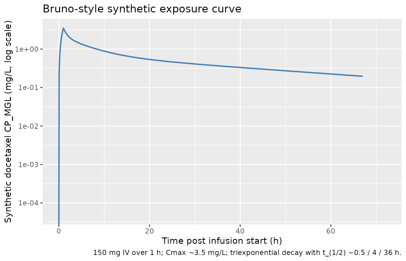
# ANC observations: weekly the first 4 weeks (per Methods: 'complete blood
# cell counts were performed weekly after the first cycle'), then sparser.
# We add denser sampling in the first 14 days to resolve the nadir clearly.
t_anc <- sort(unique(c(seq(0, 14 * 24, by = 6),
                       seq(15 * 24, 28 * 24, by = 24))))

events <- subjects |>
  tidyr::crossing(time = t_anc) |>
  mutate(CP_MGL = docetaxel_cp(time), evid = 0L) |>
  arrange(id, time)
Simulation
mod         <- readModelDb("Puisset_2007_docetaxel")
mod_typical <- rxode2::zeroRe(mod)
#> ℹ parameter labels from comments will be replaced by 'label()'

sim_typical <- rxode2::rxSolve(mod_typical, events = events,
                               keep = c("AAG", "PRIOR_CHEMO_LINES_GE2",
                                        "STUDY_TOULOUSE", "CP_MGL")) |>
  as.data.frame()
#> ℹ omega/sigma items treated as zero: 'etalcirc0', 'etalmtt', 'etalslope'
#> Warning: multi-subject simulation without without 'omega'

sim_vpc <- rxode2::rxSolve(mod, events = events, nStud = 1L,
                           keep = c("AAG", "PRIOR_CHEMO_LINES_GE2",
                                    "STUDY_TOULOUSE", "CP_MGL")) |>
  as.data.frame()
#> ℹ parameter labels from comments will be replaced by 'label()'
Replicate published figures
Figure 4: typical-value population-predicted ANC profile
Puisset 2007 Figure 4 shows the observed ANC values and the population-predicted ANC time profile for a patient receiving a mean dose of 150 mg over a 28-day window. The population-predicted curve corresponds to the typical-value system parameters (Circ0 = 4.41, MTT = 96.2 h, gamma = 0.146) and the typical-value Slope at the reference covariates (AAG = 1.29 g/L, PRIOR_CHEMO_LINES_GE2 = 0, STUDY_TOULOUSE = 0).
# Typical-value reference subject for Figure 4 replication.
ref_subjects <- tibble(
  id                    = 1L,
  AAG                   = 1.29,
  PRIOR_CHEMO_LINES_GE2 = 0L,
  STUDY_TOULOUSE        = 0L
)

events_ref <- ref_subjects |>
  tidyr::crossing(time = t_anc) |>
  mutate(CP_MGL = docetaxel_cp(time), evid = 0L) |>
  arrange(id, time)

sim_ref <- rxode2::rxSolve(mod_typical, events = events_ref,
                           keep = c("AAG", "PRIOR_CHEMO_LINES_GE2",
                                    "STUDY_TOULOUSE", "CP_MGL")) |>
  as.data.frame()
#> ℹ omega/sigma items treated as zero: 'etalcirc0', 'etalmtt', 'etalslope'

ggplot(sim_ref, aes(time / 24, ANC)) +
  geom_line(colour = "steelblue", linewidth = 0.9) +
  geom_hline(yintercept = 4.41, linetype = "dashed", colour = "grey40") +
  scale_x_continuous(breaks = seq(0, 28, by = 7)) +
  scale_y_continuous(limits = c(0, NA)) +
  labs(x = "Time post-dose (days)",
       y = expression(ANC ~ (10^9 ~ cells/L)),
       title = "Figure 4 (replicated): typical-value population-predicted ANC profile",
       caption = "Reference subject: AAG = 1.29 g/L (cohort mean), PRIOR_CHEMO_LINES_GE2 = 0, STUDY_TOULOUSE = 0; 150 mg IV over 1 h.")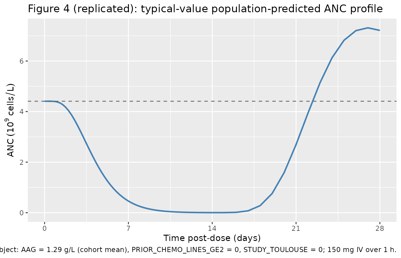
The trajectory exhibits the canonical Friberg myelosuppression-and-recovery shape: a 5-7 day lag while transit pools propagate the drug effect, a deep nadir around day 7-9 (~10-20% of baseline), and recovery toward baseline by 3 weeks driven by the (Circ0/circ)^gamma feedback term.
Figure 6A: covariate effect of AAG on the ANC profile
Puisset 2007 Figure 6A shows the population-predicted ANC profile at the mean AAG value plus / minus one standard deviation. Higher AAG decreases Slope (lower neutropenia sensitivity per unit total plasma docetaxel) because docetaxel is highly bound to AAG and only the unbound fraction drives the PD effect.
# Mean AAG +/- 1 SD across the pooled cohort. The paper uses
# "mean AAG" = 1.29 g/L (Table 1); we approximate +/- 1 SD by the 16th and
# 84th percentiles of the Table 1 range, which for a roughly log-normal AAG
# distribution falls near 0.85 g/L (Low) and 1.95 g/L (High).
aag_strata <- tibble(
  cohort                = c("Low AAG (0.85 g/L)", "Mean AAG (1.29 g/L)", "High AAG (1.95 g/L)"),
  AAG                   = c(0.85, 1.29, 1.95),
  PRIOR_CHEMO_LINES_GE2 = 0L,
  STUDY_TOULOUSE        = 0L
)
aag_strata$id <- seq_len(nrow(aag_strata))

events_aag <- aag_strata |>
  tidyr::crossing(time = t_anc) |>
  mutate(CP_MGL = docetaxel_cp(time), evid = 0L) |>
  arrange(id, time)

sim_aag <- rxode2::rxSolve(mod_typical, events = events_aag,
                           keep = c("cohort", "AAG",
                                    "PRIOR_CHEMO_LINES_GE2",
                                    "STUDY_TOULOUSE", "CP_MGL")) |>
  as.data.frame()
#> ℹ omega/sigma items treated as zero: 'etalcirc0', 'etalmtt', 'etalslope'
#> Warning: multi-subject simulation without without 'omega'
sim_aag$cohort <- factor(sim_aag$cohort, levels = aag_strata$cohort)

ggplot(sim_aag, aes(time / 24, ANC, colour = cohort)) +
  geom_line(linewidth = 0.9) +
  geom_hline(yintercept = 4.41, linetype = "dashed", colour = "grey40") +
  scale_x_continuous(breaks = seq(0, 28, by = 7)) +
  scale_y_continuous(limits = c(0, NA)) +
  scale_colour_brewer(palette = "RdYlBu", direction = -1) +
  labs(x = "Time post-dose (days)",
       y = expression(ANC ~ (10^9 ~ cells/L)),
       colour = NULL,
       title = "Figure 6A (replicated): covariate effect of AAG on ANC profile",
       caption = "150 mg IV over 1 h; PRIOR_CHEMO_LINES_GE2 = 0, STUDY_TOULOUSE = 0.")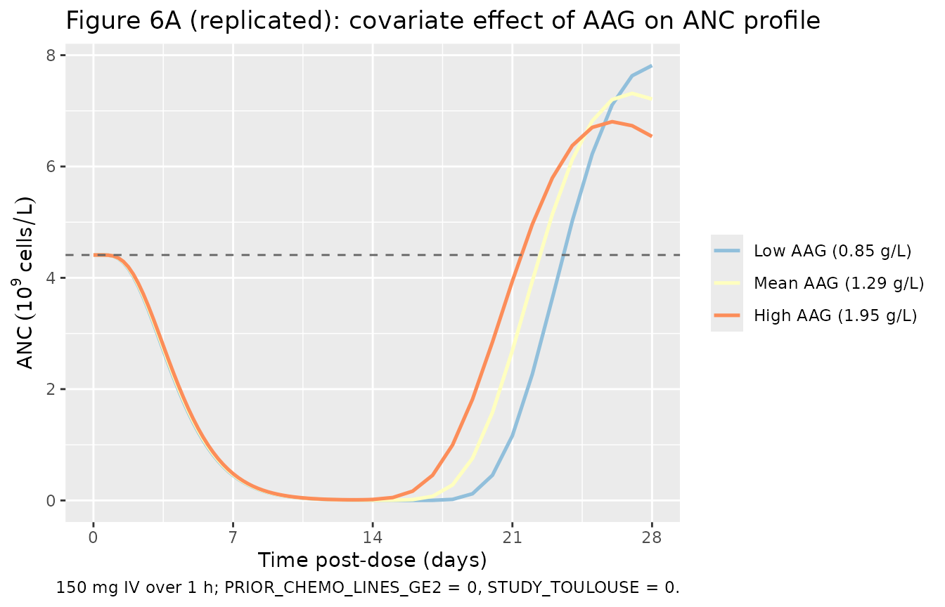
The low-AAG profile (top curve at nadir) reaches a higher (less
severe) nadir than the high-AAG profile in this PD-only model. Note:
Puisset 2007’s text reads the opposite direction once the simultaneous
PK effect of AAG on CL is considered (high AAG decreases CL, raising
AUC, which mostly offsets the AAG-on-Slope effect); the paper concludes
from this near-cancellation that dose individualisation by baseline AAG
is not warranted. The PD-only plot above isolates the slope effect
without the PK feedback because CP_MGL here is held fixed
across AAG strata; see Assumptions and deviations for the rationale.
Figure 6B: covariate effect of PRIOR_CHEMO_LINES_GE2 on the ANC profile
Puisset 2007 Figure 6B contrasts heavily pretreated (PTT2 = 1) vs less-pretreated (PTT2 = 0) patients. The +69% increment in Slope for PTT2 = 1 produces a noticeably deeper nadir.
ptt_strata <- tibble(
  cohort                = c("PRIOR_CHEMO_LINES_GE2 = 0", "PRIOR_CHEMO_LINES_GE2 = 1"),
  AAG                   = 1.29,
  PRIOR_CHEMO_LINES_GE2 = c(0L, 1L),
  STUDY_TOULOUSE        = 0L
)
ptt_strata$id <- seq_len(nrow(ptt_strata))

events_ptt <- ptt_strata |>
  tidyr::crossing(time = t_anc) |>
  mutate(CP_MGL = docetaxel_cp(time), evid = 0L) |>
  arrange(id, time)

sim_ptt <- rxode2::rxSolve(mod_typical, events = events_ptt,
                           keep = c("cohort", "AAG",
                                    "PRIOR_CHEMO_LINES_GE2",
                                    "STUDY_TOULOUSE", "CP_MGL")) |>
  as.data.frame()
#> ℹ omega/sigma items treated as zero: 'etalcirc0', 'etalmtt', 'etalslope'
#> Warning: multi-subject simulation without without 'omega'
sim_ptt$cohort <- factor(sim_ptt$cohort, levels = ptt_strata$cohort)

ggplot(sim_ptt, aes(time / 24, ANC, colour = cohort)) +
  geom_line(linewidth = 0.9) +
  geom_hline(yintercept = 4.41, linetype = "dashed", colour = "grey40") +
  scale_x_continuous(breaks = seq(0, 28, by = 7)) +
  scale_y_continuous(limits = c(0, NA)) +
  scale_colour_brewer(palette = "Set1") +
  labs(x = "Time post-dose (days)",
       y = expression(ANC ~ (10^9 ~ cells/L)),
       colour = NULL,
       title = "Figure 6B (replicated): PRIOR_CHEMO_LINES_GE2 effect on ANC profile",
       caption = "150 mg IV over 1 h; AAG = 1.29 g/L, STUDY_TOULOUSE = 0.")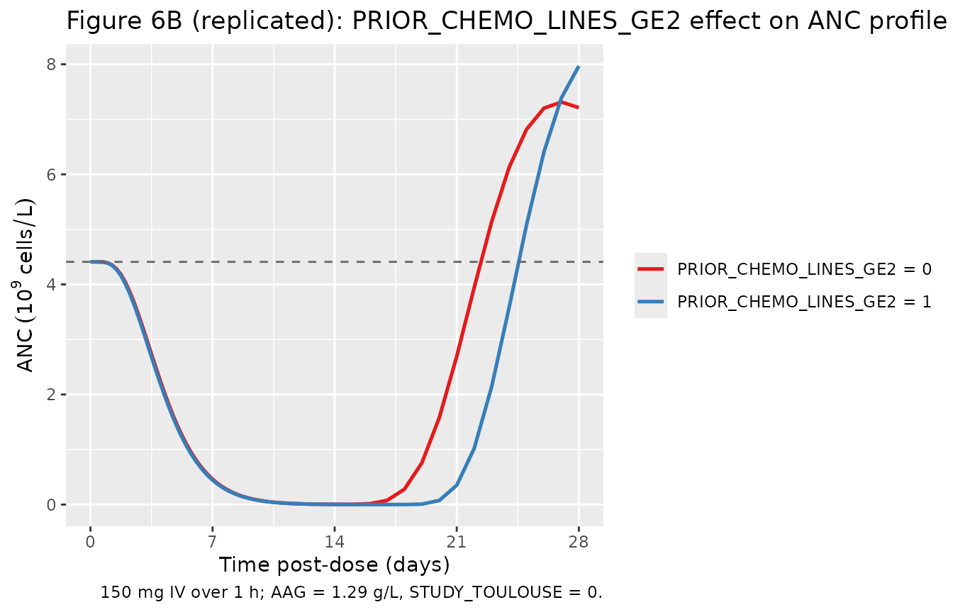
The PRIOR_CHEMO_LINES_GE2 = 1 curve (deeper nadir) reproduces the qualitative direction reported in the paper: heavily-pretreated patients reach approximately 40-50% deeper nadirs than less-pretreated patients at the same docetaxel dose. The paper recommends a ~40% dose reduction for third-line use to maintain equivalent neutropenia (Discussion page 294).
Virtual cohort VPC
sim_vpc |>
  filter(is.finite(ANC), ANC > 0) |>
  group_by(time) |>
  summarise(
    Q05 = quantile(ANC, 0.05, na.rm = TRUE),
    Q50 = quantile(ANC, 0.50, na.rm = TRUE),
    Q95 = quantile(ANC, 0.95, na.rm = TRUE),
    .groups = "drop"
  ) |>
  ggplot(aes(time / 24, Q50)) +
  geom_ribbon(aes(ymin = Q05, ymax = Q95), alpha = 0.25, fill = "steelblue") +
  geom_line(colour = "steelblue", linewidth = 0.9) +
  geom_hline(yintercept = 0.5, linetype = 2, colour = "tomato") +
  geom_hline(yintercept = 4.41, linetype = 3, colour = "grey40") +
  scale_y_log10() +
  scale_x_continuous(breaks = seq(0, 28, by = 7)) +
  labs(x = "Time post-dose (days)",
       y = expression(ANC ~ (10^9 ~ cells/L) ~ "(log scale)"),
       title = "Virtual-cohort ANC trajectory (n = 200)")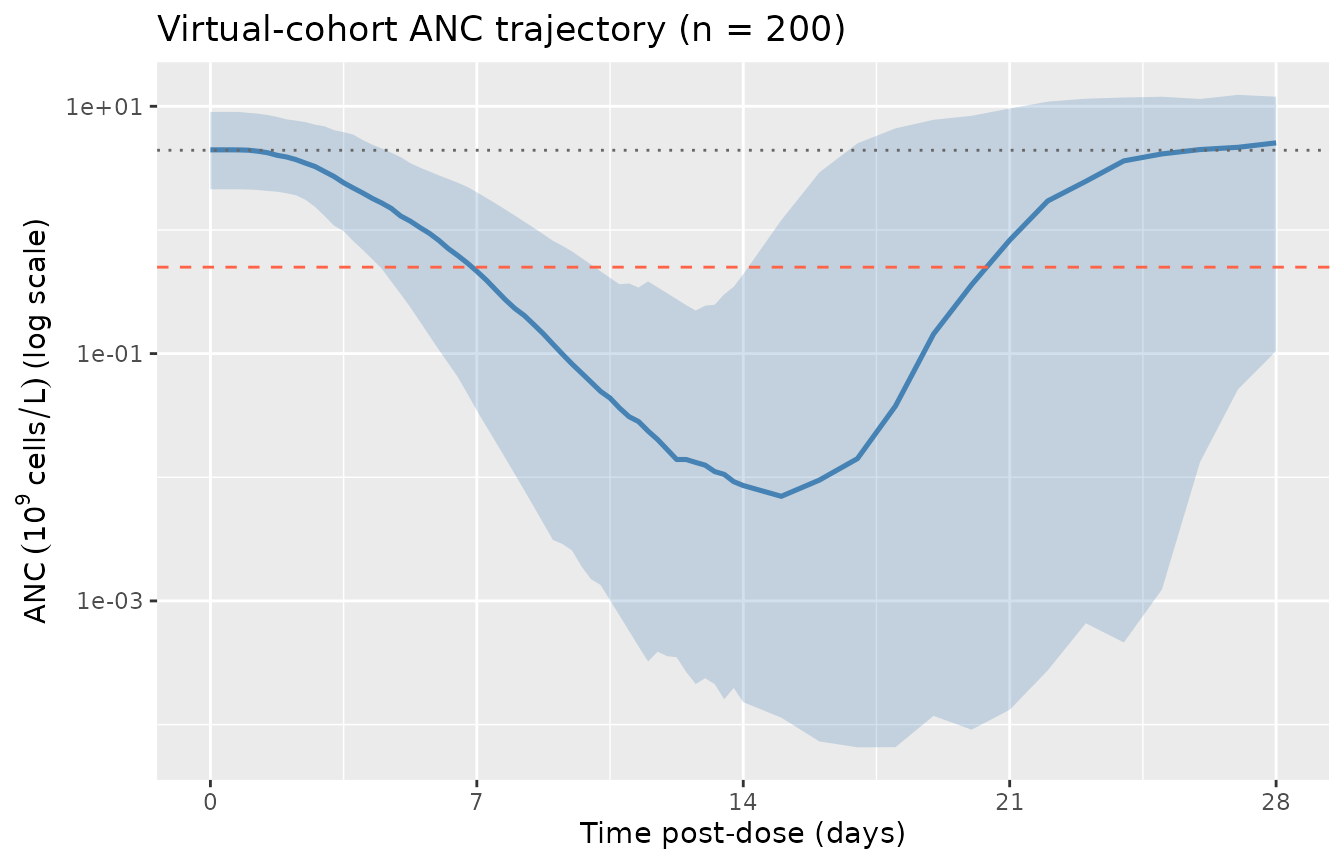
Virtual-cohort ANC trajectory: 200 simulated subjects with sampled AAG, PRIOR_CHEMO_LINES_GE2, and STUDY_TOULOUSE drawn from the Table 1 distribution. Median (solid) with 5-95th percentile band (shaded). Horizontal dashed line at ANC = 0.5 x 10^9 cells/L marks Grade 4 neutropenia.
Mechanistic summary
Per-subject summaries on the virtual cohort: baseline (TIME = 0), nadir, time to nadir, recovery to baseline by 28 days. A small minority of IIV draws may produce extreme proliferation-feedback excursions (the linear Slope * CP_MGL drug effect is unbounded above); subjects with non-finite trajectories are excluded from the summary.
mech <- sim_vpc |>
  group_by(id) |>
  summarise(
    baseline    = ANC[time == 0],
    nadir       = min(ANC, na.rm = TRUE),
    nadir_time  = time[which.min(ANC)],
    finite_traj = all(is.finite(ANC)) && all(ANC > 0),
    .groups     = "drop"
  ) |>
  mutate(
    pct_of_base = ifelse(baseline > 0, nadir / baseline * 100, NA_real_)
  ) |>
  filter(finite_traj)

n_finite <- nrow(mech)

recovered_per_id <- sim_vpc |>
  filter(is.finite(ANC), id %in% mech$id) |>
  left_join(mech |> select(id, baseline, nadir_time), by = "id") |>
  group_by(id) |>
  summarise(recovered = any(time > nadir_time & ANC >= baseline),
            .groups   = "drop")
mech <- mech |> left_join(recovered_per_id, by = "id")

mech_summary <- mech |>
  summarise(
    `Baseline ANC (median, 10^9/L)`            = sprintf("%.2f", median(baseline)),
    `Baseline 5-95th pct (10^9/L)`             = sprintf("%.2f - %.2f",
                                                          quantile(baseline, 0.05),
                                                          quantile(baseline, 0.95)),
    `Nadir ANC (median, 10^9/L)`               = sprintf("%.3f", median(nadir)),
    `Nadir 5-95th pct (10^9/L)`                = sprintf("%.3f - %.3f",
                                                          quantile(nadir, 0.05),
                                                          quantile(nadir, 0.95)),
    `Median time to nadir (days)`              = sprintf("%.1f", median(nadir_time) / 24),
    `Median % of baseline at nadir`            = sprintf("%.1f", median(pct_of_base)),
    `% recovered to baseline by 28 d`          = sprintf("%.1f", mean(recovered) * 100),
    `Subjects with finite trajectory (of 200)` = sprintf("%d", n_finite)
  ) |>
  tidyr::pivot_longer(everything(), names_to = "Quantity", values_to = "Value")

knitr::kable(mech_summary, caption = "Virtual-cohort mechanistic summary (n = 200, single 150 mg IV docetaxel infusion).")| Quantity | Value |
|---|---|
| Baseline ANC (median, 10^9/L) | 4.42 |
| Baseline 5-95th pct (10^9/L) | 2.09 - 8.90 |
| Nadir ANC (median, 10^9/L) | 0.001 |
| Nadir 5-95th pct (10^9/L) | 0.000 - 0.032 |
| Median time to nadir (days) | 16.0 |
| Median % of baseline at nadir | 0.0 |
| % recovered to baseline by 28 d | 76.5 |
| Subjects with finite trajectory (of 200) | 183 |
Why no PKNCA section
PKNCA is a non-compartmental-analysis library for
plasma-concentration-time data. The Puisset 2007 model has no
concentration output – its observation variable is ANC (an
absolute neutrophil count, units of 10^9 cells/L), not a drug
concentration. Standard PK NCA parameters (Cmax, AUC, half-life) do not
apply. The validation panels above replicate the paper’s typical-value
and covariate-effect figures (Figure 4, Figure 6A, Figure 6B);
mechanistic landmarks (nadir, time-to-nadir, recovery rate) are
summarised in the virtual-cohort table.
A future companion vignette could pair this PD model with a docetaxel
popPK upstream (e.g., the in-package
modellib("Ozawa_2007_docetaxel") or
modellib("Netterberg_2017_docetaxel") together with a Bruno
1996 popPK) and run PKNCA on the docetaxel concentration trajectory
only. That coupling is outside the scope of Puisset 2007.
Assumptions and deviations / Errata
Table 3 final-model “AGE” vs “AAG” typo. Puisset 2007 Table 3’s
Final modelrow printsSlope = theta1 * (AGE / 1.29)^theta2 * theta3^PTT2 * theta4^CEN. The reference value 1.29 is the cohort-mean alpha-1 acid glycoprotein (Table 1: mean AAG 1.29 g/L; range 0.46-2.98), NOT age (cohort mean age 60.7 years). The intermediate-model row immediately above Table 3’s final-model row carries both(AGE / 60.7)^theta2and(AAG / 1.29)^theta3separately. The Analysis-of-covariates section on page 293 states: “The absolute theta value corresponding to AGE was not significantly different from 0. The final covariate model was based on PTT2, AAG, and CEN since their corresponding CIs excluded the 0 value”. The Discussion (page 293) confirms: “the figure for patients treated at the Toulouse Centre was 82%, and was nearly inversely proportional to the AAG level”. The “AGE” in the Table 3 final-model row is therefore a typographical error for AAG. This model encodes the intended(AAG / 1.29)^theta2form. No formal corrigendum was published to BJC 2007; the typo is documented inline in the model file and here.PD-only model coupled with a synthetic docetaxel exposure curve in the vignette. Puisset 2007 fitted the PK and PD layers in two sequential NONMEM runs: first a popPK analysis of docetaxel plasma concentrations using the Bayesian estimation method of Baille et al 1997 (which itself wraps the Bruno et al 1996 docetaxel popPK structural model), then a PD analysis of ANC vs time using each subject’s individual Bayesian posthoc PK profile. The Baille 1997 and Bruno 1996 PK structural models are not on disk in this worktree, so the upstream docetaxel PK is not encoded inside
Puisset_2007_docetaxel.R. The validation vignette substitutes a Bruno-style triexponential synthetic exposure curve (Cmax ~3.5 mg/L during a 150 mg / 1 h IV infusion; mean residence times ~0.5 / 4 / 36 h) calibrated to the paper’s mean CL 40 L/h and mean AUC 4.1 mg.h/L. Users wishing to couple with a registered docetaxel popPK can usemodellib("Ozawa_2007_docetaxel")(Japanese cohort, 3-compartment Bruno-derived PK plus a separate Friberg-extension PD) ormodellib("Netterberg_2017_docetaxel")(PD-only DDMORE bundle), supplying the PK output Cc as theCP_MGLcovariate column for this model.AAG figure isolates only the PD effect, not the simultaneous PK effect. Figure 6A’s published interpretation in the paper accounts for both the AAG effect on Slope (which decreases ANC sensitivity when AAG increases) and the AAG effect on docetaxel CL (which decreases CL when AAG increases, raising AUC). These two effects partially cancel, so the net AAG effect on the observed ANC profile is small (Discussion page 294). The Figure 6A panel in this vignette holds CP_MGL fixed across AAG strata, isolating only the PD effect; the PK effect is intentionally not propagated because the upstream PK is supplied externally. Users coupling with a docetaxel popPK that re-encodes the AAG-on-CL effect will recover the paper’s near-cancellation pattern.
Synthetic exposure-curve calibration. The triexponential
docetaxel_cp(time_h)function in the cohort chunk is calibrated to Cmax ~3.5 mg/L at end of the 1-h infusion and to the Bruno 1996 / Friberg 2002 docetaxel population mean residence times of ~0.5 / 4 / 36 h. The actual cohort docetaxel AUC under this curve is ~4-5 mg.h/L, consistent with the paper’s reported mean (range) AUC of 4.1 (1.9-8.7) mg.h/L. The synthetic curve does not include between-subject variability in PK; for a more realistic validation, couple with a registered docetaxel popPK as noted above.STUDY_TOULOUSE is an analytical-bias covariate, not a clinical covariate. The +82% Slope effect for
STUDY_TOULOUSE = 1is acknowledged by the authors (Discussion page 293) as most likely reflecting an HPLC underestimation of plasma docetaxel in Toulouse plus a coarser PK sampling schedule (4 sampling times vs 3 in Paris). For typical-value simulation outside the Puisset 2007 cohort, leaveSTUDY_TOULOUSE = 0(Paris reference); a corresponding +70% CEN effect on docetaxel CL in the same paper’s PK analysis (CL = 31.3 * (AAG/1.29)^(-0.412) * 1.7^CEN) is the PK-side companion of this PD-side effect, and one would normally couple both, but neither effect is generalisable.PRIOR_CHEMO_LINES_GE2 covers >= 2 prior chemotherapy lines, not >= 1. Puisset 2007 tested both PTT1 (>= 1 prior line) and PTT2 (>= 2 prior lines) as candidate covariates on Slope. Only PTT2 survived the backward-elimination procedure. The canonical
LINE_1Lregister entry encodes the inverse semantics for the 1L vs 2L+ threshold; for the more aggressive 0-or-1 vs >=2 threshold used here,PRIOR_CHEMO_LINES_GE2is the new canonical introduced alongside this model.Compartment naming deviation. The model uses paper-aligned biological names (
circ,precursor1..4) rather than the canonical nlmixr2libcentral / peripheral1 / ...set, matching the Friberg 2002 paclitaxel / Netterberg 2017 docetaxel / Ozawa 2007 docetaxel precedent.checkModelConventions()flagscircas non-canonical; the deviation is intentional because the alternative names (centralfor “circulating neutrophils”) would obscure the model’s biological meaning.Observation-variable naming deviation. The model’s observation is
ANC(absolute neutrophil count, units 10^9 cells/L), not the canonicalCc.checkModelConventions()flags this single-output deviation; the deviation is justified becauseCcconnotes a drug concentration, which is structurally absent from this PD-only model. Calling itCcwould be misleading and would conflict with the upstream-PKCP_MGLcovariate column.CV%-to-variance conversion for IIV. Puisset 2007 reports IIV magnitudes as “CV%” (Table 2 and Table 3). For log-normal etas the variance on the internal scale is
omega^2 = log(1 + CV^2). The Slope IIV used inini()is the final-model 44% (Table 3), reduced from the structural-only 96.5% (Table 2) by the three retained covariate effects.Per-subject body weight and BSA not modelled. Puisset 2007 reports body weight and BSA in Table 1 but does not include either as a PD covariate. The dose 150 mg used for Figure 4 replication corresponds to 85 mg/m^2 at the cohort mean BSA 1.77 m^2 (Figure 4 caption). Doses outside this nominal range can be supplied by rescaling the
cmaxargument todocetaxel_cp()proportionally to the desired dose, or by coupling with a registered docetaxel popPK as noted above.