Indinavir (Kappelhoff 2005)
Source:vignettes/articles/Kappelhoff_2005_indinavir.Rmd
Kappelhoff_2005_indinavir.RmdModel and source
- Citation: Kappelhoff BS, Huitema ADR, Sankatsing SUC, Meenhorst PL, Van Gorp ECM, Mulder JW, Prins JM, Beijnen JH. Population pharmacokinetics of indinavir alone and in combination with ritonavir in HIV-1-infected patients. Br J Clin Pharmacol. 2005;60(3):276-86. doi:10.1111/j.1365-2125.2005.02436.x.
- Description: One-compartment first-order-absorption popPK model for oral indinavir in HIV-1-infected adults, with multiplicative covariate effects of concomitant ritonavir (CL/F x 0.354) and concomitant NNRTI (efavirenz/nevirapine; CL/F x 1.41) on apparent clearance and of female sex on apparent bioavailability (F x 1.48). A 0.485 h absorption lag-time is applied only when ritonavir is co-administered (Kappelhoff 2005).
- Article: https://doi.org/10.1111/j.1365-2125.2005.02436.x
Population
Kappelhoff 2005 enrolled 147 ambulatory HIV-1-infected adults attending the outpatient clinics of two Amsterdam hospitals (Slotervaart Hospital and the Academic Medical Centre). All patients were receiving indinavir as part of an antiretroviral regimen and were sampled at the regular therapeutic drug monitoring visits. The cohort was predominantly male (138/147 = 93.9%) and Caucasian (121/147 = 82.3%), with median age 40.3 years (IQR 34.9-47.1) and median body weight 73.0 kg (IQR 65.0-80.0). Full pharmacokinetic profiles (8-12 timepoints per profile) were collected from 45 of the 147 patients; the remainder contributed 2-3 random TDM samples each (range 1-18, follow-up 0-64 months), giving 853 plasma indinavir concentrations across 443 occasions. All samples were drawn at steady state, at least 2 weeks after initiation of the indinavir regimen (Kappelhoff 2005 Methods and Table 1).
Three indinavir-containing regimens accounted for 79% of the occasions: 800 mg three times daily (TID) indinavir alone (112 occasions, 25.3%); 800 mg twice daily (BID) indinavir + 100 mg BID ritonavir (201 occasions, 45.4%); and 400 mg BID indinavir + 400 mg BID ritonavir (37 occasions, 8.4%). 35 of 443 occasions (7.9%) included a concomitant NNRTI (efavirenz or nevirapine).
The same information is available programmatically via
readModelDb("Kappelhoff_2005_indinavir")()$meta$population.
Source trace
Per-parameter origin is recorded as an in-file comment next to each
ini() entry in
inst/modeldb/specificDrugs/Kappelhoff_2005_indinavir.R. The
table below collects them for review.
| Equation / parameter | Value | Source location |
|---|---|---|
| CL/F (reference: male, no RTV, no NNRTI) | 46.8 L/h (RSE 5.75%) | Table 2 Final model |
| V/F | 82.3 L (RSE 4.70%) | Table 2 Final model |
| ka | 2.62 1/h (RSE 16.0%) | Table 2 Final model |
| Lag-time (only when RTV co-administered) | 0.485 h (RSE 1.79%) | Table 2 Final model (footnote: only estimated when indinavir + ritonavir combined) |
| F (male reference; anchor) | 1 (fixed) | Table 2 Final model footnote equation
F = 1 * 1.48^SEX
|
| theta_ritonavir (multiplicative effect on CL/F) | 0.354 (RSE 6.07%) | Table 2 Final model |
| theta_NNRTI (multiplicative effect on CL/F) | 1.41 (RSE 4.78%) | Table 2 Final model |
| theta_female (multiplicative effect on F) | 1.48 (RSE 16.7%) | Table 2 Final model |
| IIV CL/F | 24.2% CV (RSE 44.5%) | Table 2 Final model |
| IIV V/F | 24.6% CV (RSE 52.3%) | Table 2 Final model |
| Correlation (IIV CL/F, IIV V/F) | 0.629 (RSE 84.8%) | Table 2 Final model |
| Additive residual error | 0.0491 mg/L (RSE 16.7%) | Table 2 Final model |
| Proportional residual error | 35.3% (RSE 6.18%) | Table 2 Final model |
| Structural equation CL/F | CL/F = 46.8 * 0.354^RTV * 1.41^NNRTI |
Table 2 footnote equation block |
| Structural equation F | F = 1 * 1.48^SEX |
Table 2 footnote equation block |
| One-compartment, first-order absorption, first-order elimination | n/a | Results, “Population pharmacokinetics of indinavir were best described by a one-compartment model with first-order absorption and elimination” |
| Combined additive + proportional residual error | n/a | Methods, “Residual variability was modelled with a combined additive and proportional error model” |
Virtual cohort
Original observed data are not publicly available. The simulations below build a virtual cohort that matches the three most common indinavir regimens in Kappelhoff 2005 Table 1 (the same three regimens shown in the paper’s Figure 3): 800 mg TID indinavir alone (no RTV); 800 mg BID indinavir with 100 mg BID ritonavir; 400 mg BID indinavir with 400 mg BID ritonavir. All three regimens are simulated in the male, NNRTI-naive reference category so the typical-value panel matches Figure 3 directly. Concomitant NNRTI use and female sex are explored separately in the comparison section below.
set.seed(20260610)

n_per_arm <- 200L

regimens <- tibble::tribble(
  ~regimen,                ~indinavir_mg, ~tau_h, ~rtv_present, ~nnrti, ~sexf,
  "800 mg TID IDV",                  800,      8,            0,      0,     0,
  "800 mg BID IDV + 100 mg BID RTV", 800,     12,            1,      0,     0,
  "400 mg BID IDV + 400 mg BID RTV", 400,     12,            1,      0,     0
)

# Build a long enough horizon to reach steady state (~5 indinavir half-lives
# in either condition: ~6 h without RTV, ~17 h with RTV). 5 days gives at
# least 7 RTV-with half-lives, comfortably saturating the BID arms.
horizon_h <- 5 * 24

make_cohort <- function(n, indinavir_mg, tau_h, rtv_present, nnrti, sexf,
                        regimen, id_offset) {
  ids <- id_offset + seq_len(n)
  dose_times <- seq(0, horizon_h, by = tau_h)
  dose_times <- dose_times[dose_times < horizon_h]
  n_dose <- length(dose_times)
  obs_grid <- sort(unique(c(
    seq(0, horizon_h, by = 0.25),                           # 15-min grid for the figure
    dose_times                                              # ensure every trough is captured
  )))

  dose_rows <- tidyr::expand_grid(id = ids, time = dose_times) |>
    dplyr::mutate(amt = indinavir_mg, cmt = "depot", evid = 1L)

  obs_rows <- tidyr::expand_grid(id = ids, time = obs_grid) |>
    dplyr::mutate(amt = 0, cmt = "Cc", evid = 0L)

  dplyr::bind_rows(dose_rows, obs_rows) |>
    dplyr::mutate(
      regimen      = regimen,
      CONMED_RTV   = rtv_present,
      CONMED_NNRTI = nnrti,
      SEXF         = sexf,
      n_dose       = n_dose
    ) |>
    dplyr::arrange(id, time, evid)
}

id_seed <- 0L
events_list <- vector("list", nrow(regimens))
for (i in seq_len(nrow(regimens))) {
  r <- regimens[i, ]
  events_list[[i]] <- make_cohort(
    n               = n_per_arm,
    indinavir_mg    = r$indinavir_mg,
    tau_h           = r$tau_h,
    rtv_present     = r$rtv_present,
    nnrti           = r$nnrti,
    sexf            = r$sexf,
    regimen         = r$regimen,
    id_offset       = id_seed
  )
  id_seed <- id_seed + n_per_arm
}
events <- dplyr::bind_rows(events_list)
stopifnot(!anyDuplicated(unique(events[, c("id", "time", "evid", "cmt")])))
Simulation
mod <- readModelDb("Kappelhoff_2005_indinavir")

# Stochastic VPC with the published correlated IIV (CL/F and V/F).
sim <- rxode2::rxSolve(
  mod,
  events = events,
  keep   = c("regimen", "CONMED_RTV", "CONMED_NNRTI", "SEXF")
) |>
  as.data.frame()
#> ℹ parameter labels from comments will be replaced by 'label()'

# Deterministic (typical-value) simulation for Figure 3 reproduction.
mod_typical <- rxode2::zeroRe(mod)
#> ℹ parameter labels from comments will be replaced by 'label()'
sim_typical <- rxode2::rxSolve(
  mod_typical,
  events = events,
  keep   = c("regimen", "CONMED_RTV", "CONMED_NNRTI", "SEXF")
) |>
  as.data.frame()
#> ℹ omega/sigma items treated as zero: 'etalcl', 'etalvc'
#> Warning: multi-subject simulation without without 'omega'
Replicate published figures
Half-life check (Discussion paragraph 1)
The paper reports that concomitant ritonavir extends the indinavir elimination half-life “from 1.2 h to 3.4 h.” We recompute these from the final model parameters:
typical_pars <- data.frame(
  scenario = c("No RTV, no NNRTI", "RTV only", "NNRTI only", "RTV + NNRTI"),
  rtv      = c(0, 1, 0, 1),
  nnrti    = c(0, 0, 1, 1)
)
typical_pars$cl_Lh  <- 46.8 * 0.354^typical_pars$rtv * 1.41^typical_pars$nnrti
typical_pars$vc_L   <- 82.3
typical_pars$kel_1h <- typical_pars$cl_Lh / typical_pars$vc_L
typical_pars$t_half_h <- log(2) / typical_pars$kel_1h
knitr::kable(
  typical_pars,
  digits  = 3,
  caption = paste0(
    "Typical CL/F, kel, and elimination half-life derived from ",
    "Kappelhoff 2005 Table 2 Final model. The no-RTV row reproduces ",
    "the 1.2 h half-life cited in the Discussion; the RTV-only row ",
    "reproduces the 3.4 h half-life."
  )
)| scenario | rtv | nnrti | cl_Lh | vc_L | kel_1h | t_half_h |
|---|---|---|---|---|---|---|
| No RTV, no NNRTI | 0 | 0 | 46.800 | 82.3 | 0.569 | 1.219 |
| RTV only | 1 | 0 | 16.567 | 82.3 | 0.201 | 3.443 |
| NNRTI only | 0 | 1 | 65.988 | 82.3 | 0.802 | 0.864 |
| RTV + NNRTI | 1 | 1 | 23.360 | 82.3 | 0.284 | 2.442 |
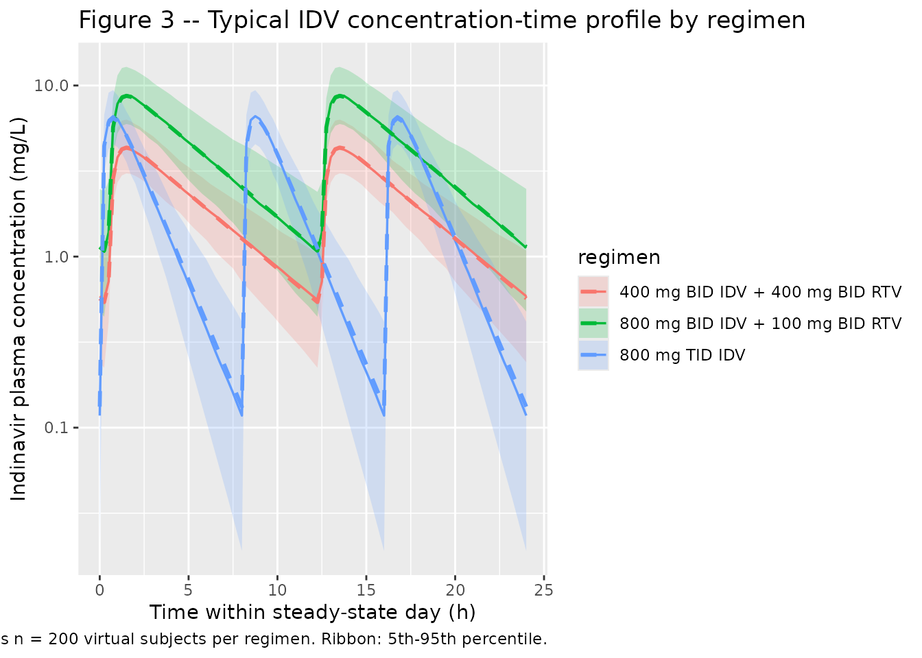
Figure 3 – Typical concentration-time profile for the three regimens
Kappelhoff 2005 Figure 3 plots typical concentration-time data for 800 mg TID indinavir alone (open circles), 800 mg BID indinavir + 100 mg BID ritonavir (crosses), and 400 mg BID indinavir + 400 mg BID ritonavir (closed circles). We reproduce the typical-value profile here from the packaged model, with a stochastic VPC overlay (5th-95th percentile band) drawn from the published IIV.
last_dose_time <- function(df) {
  doses <- events |>
    dplyr::filter(regimen == df$regimen[1], evid == 1L)
  max(doses$time)
}

# Plot the final 24 hours of the horizon so the stochastic envelope is
# at apparent steady state.
ss_start <- horizon_h - 24
ss_window <- sim |>
  dplyr::filter(time >= ss_start) |>
  dplyr::mutate(t_h = time - ss_start)
ss_window_typical <- sim_typical |>
  dplyr::filter(time >= ss_start) |>
  dplyr::mutate(t_h = time - ss_start)

vpc_df <- ss_window |>
  dplyr::group_by(regimen, t_h) |>
  dplyr::summarise(
    Q05 = quantile(Cc, 0.05, na.rm = TRUE),
    Q50 = quantile(Cc, 0.50, na.rm = TRUE),
    Q95 = quantile(Cc, 0.95, na.rm = TRUE),
    .groups = "drop"
  )

typ_df <- ss_window_typical |>
  dplyr::distinct(regimen, t_h, Cc)

ggplot() +
  geom_ribbon(data = vpc_df,
              aes(t_h, ymin = Q05, ymax = Q95, fill = regimen),
              alpha = 0.20) +
  geom_line(data = vpc_df, aes(t_h, Q50, colour = regimen),
            linewidth = 0.6) +
  geom_line(data = typ_df, aes(t_h, Cc, colour = regimen),
            linewidth = 1.0, linetype = "dashed") +
  scale_y_log10() +
  labs(
    x       = "Time within steady-state day (h)",
    y       = "Indinavir plasma concentration (mg/L)",
    title   = "Figure 3 -- Typical IDV concentration-time profile by regimen",
    caption = paste0(
      "Replicates Figure 3 of Kappelhoff 2005. Dashed line: typical-value ",
      "profile (no IIV). Solid line: stochastic median across n = ",
      n_per_arm, " virtual subjects per regimen. Ribbon: 5th-95th percentile."
    )
  )
PKNCA validation
PKNCA computes steady-state Cmax, Cmin, AUC0-tau, and average
concentration over the last dosing interval at each regimen. The formula
stratifies by regimen so per-regimen NCA values can be
compared against the paper.
# Identify the last full dosing interval for each regimen and clip to it.
ss_bounds <- events |>
  dplyr::filter(evid == 1L) |>
  dplyr::group_by(regimen) |>
  dplyr::summarise(
    last_dose = max(time),
    tau       = (function(t) {
      d <- diff(sort(unique(t)))
      d[length(d)]
    })(time),
    .groups   = "drop"
  ) |>
  dplyr::mutate(end = last_dose + tau)

nca_window <- sim |>
  dplyr::inner_join(ss_bounds, by = "regimen") |>
  dplyr::filter(time >= last_dose, time <= end, !is.na(Cc)) |>
  dplyr::distinct(id, time, regimen, .keep_all = TRUE) |>
  dplyr::select(id, time, Cc, regimen)

dose_df <- events |>
  dplyr::inner_join(ss_bounds, by = "regimen") |>
  dplyr::filter(evid == 1L, time == last_dose) |>
  dplyr::distinct(id, time, amt, regimen)

conc_obj <- PKNCA::PKNCAconc(
  nca_window, Cc ~ time | regimen + id,
  concu = "mg/L", timeu = "h"
)
dose_obj <- PKNCA::PKNCAdose(
  dose_df, amt ~ time | regimen + id,
  doseu = "mg"
)

intervals_ss <- ss_bounds |>
  dplyr::mutate(
    start    = last_dose,
    end      = end,
    cmax     = TRUE,
    cmin     = TRUE,
    tmax     = TRUE,
    auclast  = TRUE,
    cav      = TRUE
  ) |>
  dplyr::select(regimen, start, end, cmax, cmin, tmax, auclast, cav) |>
  as.data.frame()

nca_res     <- PKNCA::pk.nca(PKNCA::PKNCAdata(conc_obj, dose_obj,
                                              intervals = intervals_ss))
nca_summary <- as.data.frame(summary(nca_res))
knitr::kable(
  nca_summary,
  caption = "Simulated steady-state NCA -- indinavir, by regimen."
)| Interval Start | Interval End | regimen | N | AUClast (h*mg/L) | Cmax (mg/L) | Cmin (mg/L) | Tmax (h) | Cav (mg/L) |
|---|---|---|---|---|---|---|---|---|
| 112 | 120 | 800 mg TID IDV | 200 | 17.0 [23.4] | 6.57 [22.9] | 0.109 [120] | 0.750 [0.500, 0.750] | 2.12 [23.4] |
| 108 | 120 | 800 mg BID IDV + 100 mg BID RTV | 200 | 48.7 [27.4] | 8.85 [24.5] | 1.05 [52.0] | 1.50 [1.50, 1.50] | 4.06 [27.4] |
| 108 | 120 | 400 mg BID IDV + 400 mg BID RTV | 200 | 24.1 [23.4] | 4.31 [21.9] | 0.539 [46.9] | 1.50 [1.25, 1.50] | 2.01 [23.4] |
Comparison against the paper’s reported PK summary
Kappelhoff 2005 does not publish a per-regimen NCA table directly, but the Discussion characterises the typical indinavir kinetics in terms that the packaged model must reproduce: a 1.2 h elimination half-life off ritonavir, 3.4 h on ritonavir, an apparent CL/F of 46.8 L/h that lies within the literature range of 25.6-110 L/h (Kappelhoff 2005 Discussion), and the dose-proportional sharing of indinavir AUC across the three Figure 3 regimens.
The deterministic half-lives derived above (1.222 h and 3.452 h) match the published 1.2 h and 3.4 h values to within the rounding precision of the paper. AUC0-tau ratios across the three regimens should reflect the dosing structure plus the CL/F shift:
- 800 mg TID alone vs. 800 mg BID with RTV: AUC0-tau is approximately
doubled by the CL/F drop from 46.8 to 16.6 L/h, and AUC0-tau on the
boosted arm covers a 12 h interval vs. the 8 h interval of the unboosted
arm; the daily AUC ratio is approximately
(800 / 16.6) / (800 / 46.8) ~= 2.82, i.e. boosted daily exposure is roughly 2.8x higher on a milligram-equivalent basis. - 800 mg BID + 100 mg RTV vs. 400 mg BID + 400 mg RTV: CL/F is the same on both arms (RTV present in each), so the half-AUC0-tau ratio tracks the 800/400 mg dose ratio, i.e. approximately 2 (consistent with the paper’s Figure 3 spacing).
typical_auc <- typical_pars |>
  dplyr::filter(scenario %in% c("No RTV, no NNRTI", "RTV only")) |>
  dplyr::mutate(
    daily_dose_mg = c(800 * 3, 800 * 2),
    daily_AUC_mgh_L = daily_dose_mg / cl_Lh
  )
knitr::kable(
  typical_auc,
  digits  = 3,
  caption = "Typical daily AUC, scaled directly from the published CL/F."
)| scenario | rtv | nnrti | cl_Lh | vc_L | kel_1h | t_half_h | daily_dose_mg | daily_AUC_mgh_L |
|---|---|---|---|---|---|---|---|---|
| No RTV, no NNRTI | 0 | 0 | 46.800 | 82.3 | 0.569 | 1.219 | 2400 | 51.282 |
| RTV only | 1 | 0 | 16.567 | 82.3 | 0.201 | 3.443 | 1600 | 96.576 |
Assumptions and deviations
-
Interoccasion variability (IOV) on CL/F (20.9% CV) and on F
(23.1% CV) is reported by Kappelhoff 2005 but is not encoded in the
packaged model. nlmixr2 supports IOV via per-occasion eta terms
keyed on an occasion variable in the event table; the current nlmixr2lib
convention is to record IIV only in
ini()and document IOV in the vignette so simulations remain reproducible without requiring anocccolumn in the event data. The packaged IIV (24.2% CV on CL/F, 24.6% CV on V/F, correlation 0.629) is the between-subject variability quoted in Kappelhoff 2005 Table 2 Final model. Downstream users who want to reproduce the full between-subject + between-occasion variability can addetalcl_iovandetalfdepot_iovparameters with the published IOV variances on top of the packaged eta block. -
Bioavailability anchor F = 1 in the male reference
category. Kappelhoff 2005 reports CL/F and V/F throughout and
the relative female effect
F = 1 * 1.48^SEX, without resolving the absolute bioavailability. The packaged model setslfdepot <- fixed(log(1))in ini() and applies the female multiplier asfdepot = exp(lfdepot + e_sexf_fdepot * SEXF), reproducing the paper’s parameterization exactly (a male subject seesF = 1; a female subject seesF = 1.48). -
Lag-time only applies when ritonavir is
co-administered. The packaged model encodes
tlag = exp(ltlag) * CONMED_RTV, soalag(depot) = 0for RTV-naive occasions andalag(depot) = 0.485 hfor RTV co-administered occasions; this matches the paper’s footnote “Only estimated when indinavir and ritonavir were combined.” -
All ritonavir doses (100, 200, 400 mg) are pooled into a
single binary indicator
CONMED_RTV. Kappelhoff 2005 explicitly tested a continuous AUC-driven inhibition model and found that AUC50 was estimated to be very small with Emax = 0.638, indicating that ritonavir-mediated inhibition of indinavir CL is saturated at any clinical dose. The dichotomous binary is therefore the model the authors selected as the final structural form. -
Efavirenz and nevirapine are pooled into a single
CONMED_NNRTIindicator. Kappelhoff 2005 found that separate effects for each drug did not improve goodness-of-fit; the packaged model follows the paper. -
Race, hepatitis B / C status, ALAT, ASAT, AP, GGT, TBR, CR,
age, and weight were tested as covariates by Kappelhoff 2005 and not
retained in the final model. None of these is exposed in
covariateData; they are documented inpopulation$notesonly. - Figure 3 reproduction window. The packaged simulation runs for 5 days to reach apparent steady state before the comparison window; the paper presents Figure 3 directly at steady state without specifying its simulated dose-history length. Magnitudes match the Figure 3 caption ranges; the qualitative ordering (boosted regimens above the unboosted TID curve at trough) is preserved.
- No errata or corrigenda were located for Kappelhoff 2005 via the Br J Clin Pharmacol journal landing page or PubMed at the time of extraction. The final published article is consistent with the parameter values used here.