Model and source
- Citation: Guan X, Tang X, Zhang Y, Xie H, Luo L, Wu D, Chen R, Hu P. (2021). Population Pharmacokinetic Analysis of Yimitasvir in Chinese Healthy Volunteers and Patients With Chronic Hepatitis C Virus Infection. Front Pharmacol 11:617122. doi:10.3389/fphar.2020.617122
- Description: Two-compartment population PK model for oral yimitasvir (an HCV NS5A inhibitor) in Chinese healthy volunteers and patients with chronic HCV genotype 1 infection (Guan 2021; N = 219 across six studies), with sequential zero-order (duration Td) then first-order absorption, first-order elimination, a linear decrease in relative bioavailability of 12.9% per 100 mg above 100 mg, food effects on ka and F, sex and baseline ALT effects on CL/F, and a patient effect on Td.
- Article: https://doi.org/10.3389/fphar.2020.617122 (open access)
The article carries the volume year 2020 (Front Pharmacol volume 11) but was published on 28 January 2021 and cites itself as Guan et al. (2021); the model is named for the publication year.
Population
Guan 2021 pooled 3,540 plasma concentrations from 219 Chinese subjects in six studies (Table 1): four phase 1 studies in healthy volunteers (single ascending dose 30-600 mg, multiple ascending dose 100-400 mg once daily for 7 days, and a 100 mg fasted / high-fat-meal crossover), a phase 1b study in patients with chronic HCV genotype 1 infection (30, 100 or 200 mg once daily for 7 days, dosed in the evening at least 4 h after dinner), and a phase 2 study in patients (100 or 200 mg once daily for 12 weeks with sofosbuvir 400 mg). There were 72 healthy volunteers and 147 patients; median age 38 years (18-75), median body weight 62 kg (44-100), 42.5% female, median baseline ALT 31.6 IU/L (5.0-666) (Table 2).
The same information is available programmatically via
rxode2::rxode2(readModelDb("Guan_2021_yimitasvir"))$population.
Source trace
| Equation / parameter | Value | Source location |
|---|---|---|
| Structure: 2-compartment, sequential zero-order (Td) then first-order (ka) absorption, first-order elimination | n/a | Results ‘Model Development’; Figure 2 |
lka |
log(1.31) 1/h | Table 3 ‘Ka’ |
lcl |
log(13.8) L/h | Table 3 ‘CL/F’ |
lvc |
log(188) L | Table 3 ‘V1/F’ |
lq |
log(3.96) L/h | Table 3 ‘Q/F’ |
lvp |
log(58.6) L | Table 3 ‘V2/F’ |
ld1 |
log(2.17) h | Table 3 ‘Td’ |
lfdepot |
fixed(log(1)) | Table 3 ‘F’ = 1 (fixed); Eq. 3 theta_F |
e_dose_fdepot |
fixed(0.129) | Table 3 ‘Alpha’ (fixed); Eq. 3 |
e_meal_predose_4h_ka |
-1.71 | Table 3 ‘Ka ~ Food1’ |
e_fed_highfat_ka |
-2.40 | Table 3 ‘Ka ~ Food2’ |
e_meal_predose_4h_fdepot |
-0.341 | Table 3 ‘F ~ Food1’ |
e_fed_highfat_fdepot |
-0.485 | Table 3 ‘F ~ Food2’ |
e_sexf_cl |
-0.251 | Table 3 ‘CL/F ~ Female’ |
e_alt_cl |
-0.0950 | Table 3 ‘CL/F ~ ALT’; median 31.6 IU/L from Table 2 and Results |
e_hcv_pos_d1 |
-0.416 | Table 3 ‘Td ~ Patient’ |
etalcl, etalvc block |
SD 0.485, 0.736; correlation 0.565 | Table 3 ‘Random effect’; see ‘IIV scale’ below |
propSd |
0.305 | Table 3 ‘sigma’ |
| Covariate forms | exponential categorical, median-normalised power | Eq. 4, Eq. 5 |
| Dose on F | F = 1 - Alpha (Dose - 100)/100 above 100 mg | Eq. 3 |
Typical-value replication of Figure 5
Figure 5 of Guan 2021 is a sensitivity plot of steady-state exposure after 100 mg once daily for 12 weeks. The typical subject is a healthy male volunteer, fasted at least 10 h, ALT 31.6 IU/L; each bar changes one covariate. These are deterministic typical-value quantities, so they are compared with tight tolerances.
mod <- readModelDb("Guan_2021_yimitasvir")
ui <- rxode2::rxode2(mod)
#> ℹ parameter labels from comments will be replaced by 'label()'
# The explicit ODEs must be solved, not replaced by rxode2's linear solution
stopifnot(is.null(ui$linCmt))

scen <- tibble::tribble(
  ~scenario,          ~SEXF, ~ALT, ~HCV_POS, ~FED_HIGHFAT, ~MEAL_PREDOSE_4H,
  "Base",             0,     31.6, 0,        0,            0,
  "Fasted 4 h",       0,     31.6, 0,        0,            1,
  "High-fat",         0,     31.6, 0,        1,            0,
  "Female",           1,     31.6, 0,        0,            0,
  "ALT 9 IU/L",       0,     9,    0,        0,            0,
  "ALT 153 IU/L",     0,     153,  0,        0,            0,
  "Patient",          0,     31.6, 1,        0,            0
) |>
  mutate(id = seq_len(n()), DOSE = 100)

tau <- 24
n_dose <- 84
dose_rows <- tidyr::crossing(id = scen$id, time = seq(0, by = tau, length.out = n_dose)) |>
  mutate(evid = 1L, amt = 100, cmt = "depot", rate = -2)
obs_rows <- tidyr::crossing(id = scen$id, time = seq((n_dose - 1) * tau, n_dose * tau, by = 0.05)) |>
  mutate(evid = 0L, amt = 0, cmt = "central", rate = 0)
ev_fig5 <- bind_rows(dose_rows, obs_rows) |>
  left_join(scen, by = "id") |>
  relocate(id, time, evid, amt, cmt, rate) |>
  arrange(id, time, desc(evid))

sim_fig5 <- rxode2::rxSolve(
  rxode2::zeroRe(mod), ev_fig5,
  keep = "scenario", returnType = "data.frame", atol = 1e-10, rtol = 1e-10
)
#> ℹ parameter labels from comments will be replaced by 'label()'
#> ℹ omega/sigma items treated as zero: 'etalcl', 'etalvc'
#> Warning: multi-subject simulation without without 'omega'

fig5 <- sim_fig5 |>
  filter(time >= (n_dose - 1) * tau) |>
  group_by(scenario) |>
  arrange(time, .by_group = TRUE) |>
  summarise(
    AUCss = sum(diff(time) * (head(Cc, -1) + tail(Cc, -1)) / 2) / 1000,
    Cmaxss = max(Cc),
    Ctroughss = last(Cc),
    .groups = "drop"
  )
base <- fig5 |> filter(scenario == "Base")
fig5_pct <- fig5 |>
  filter(scenario != "Base") |>
  mutate(
    AUCss = 100 * (AUCss / base$AUCss - 1),
    Cmaxss = 100 * (Cmaxss / base$Cmaxss - 1),
    Ctroughss = 100 * (Ctroughss / base$Ctroughss - 1)
  )
# Figure 5 bar labels, in percent change from the typical subject
published_pct <- tibble::tribble(
  ~scenario,      ~AUCss_pub, ~Ctroughss_pub, ~Cmaxss_pub,
  "Fasted 4 h",   -28.9,      -10.0,          -46.1,
  "High-fat",     -38.5,      -3.52,          -58.9,
  "Female",       28.6,       54.0,           15.1,
  "ALT 9 IU/L",   -11.6,      -20.0,          -5.89,
  "ALT 153 IU/L", 16.6,       30.1,           8.52,
  "Patient",      0.01,       -2.07,          1.09
)
cmp5 <- fig5_pct |> inner_join(published_pct, by = "scenario")

tibble::tibble(
  Quantity = c("AUCss (ug*h/mL)", "Ctrough,ss (ng/mL)", "Cmax,ss (ng/mL)"),
  Simulated = signif(c(base$AUCss, base$Ctroughss, base$Cmaxss), 4),
  Published = c(7.25, 140, 540)
) |>
knitr::kable(caption = "Typical subject at steady state, 100 mg once daily (Figure 5 'Base').")| Quantity | Simulated | Published |
|---|---|---|
| AUCss (ug*h/mL) | 7.246 | 7.25 |
| Ctrough,ss (ng/mL) | 139.900 | 140.00 |
| Cmax,ss (ng/mL) | 540.900 | 540.00 |
cmp5 |>
  mutate(across(where(is.numeric), \(x) round(x, 2))) |>
  select(scenario, AUCss, AUCss_pub, Ctroughss, Ctroughss_pub, Cmaxss, Cmaxss_pub) |>
  dplyr::rename(
    "Scenario" = scenario,
    "AUCss sim (%)" = AUCss, "AUCss pub (%)" = AUCss_pub,
    "Ctrough,ss sim (%)" = Ctroughss, "Ctrough,ss pub (%)" = Ctroughss_pub,
    "Cmax,ss sim (%)" = Cmaxss, "Cmax,ss pub (%)" = Cmaxss_pub
  ) |>
knitr::kable(caption = "Percent change from the typical subject: simulated vs Figure 5 of Guan 2021.")| Scenario | AUCss sim (%) | AUCss pub (%) | Ctrough,ss sim (%) | Ctrough,ss pub (%) | Cmax,ss sim (%) | Cmax,ss pub (%) |
|---|---|---|---|---|---|---|
| ALT 153 IU/L | 16.17 | 16.60 | 30.15 | 30.10 | 8.48 | 8.52 |
| ALT 9 IU/L | -11.25 | -11.60 | -20.05 | -20.00 | -5.84 | -5.89 |
| Fasted 4 h | -28.89 | -28.90 | -9.83 | -10.00 | -46.14 | -46.10 |
| Female | 28.53 | 28.60 | 53.97 | 54.00 | 15.02 | 15.10 |
| High-fat | -38.43 | -38.50 | -3.42 | -3.52 | -58.88 | -58.90 |
| Patient | 0.00 | 0.01 | -2.08 | -2.07 | 1.10 | 1.09 |
stopifnot(
  # Base exposures: AUCss = 100 mg / 13.8 L/h exactly; Cmax and Ctrough test
  # ka, Td, V1/F, Q/F and V2/F together.
  abs(base$AUCss / 7.25 - 1) < 0.005,
  abs(base$Ctroughss / 140 - 1) < 0.01,
  abs(base$Cmaxss / 540 - 1) < 0.01,
  # Covariate bars: every one within 0.5 percentage points of the label
  # (largest gap 0.43 pp, ALT 153 IU/L AUCss, from the rounded ALT labels).
  all(abs(cmp5$AUCss - cmp5$AUCss_pub) < 0.5),
  all(abs(cmp5$Ctroughss - cmp5$Ctroughss_pub) < 0.5),
  all(abs(cmp5$Cmaxss - cmp5$Cmaxss_pub) < 0.5)
)
The Figure 5 bars for food status and sex also independently confirm
the exponential form of Eq. 5: exp(-0.485) = 0.616 gives
the 38.5% high-fat AUC decrease, and exp(0.251) = 1.285 the
28.6% higher female AUC.
IIV scale
Table 3 lists the random effects as ‘CL/F’ 0.485, ‘V1/F’ 0.736 and ‘CL/F ~ V1/F’ 0.565, and the Results describe them as inter-individual variability of 48.5% and 73.6%. If 0.485 and 0.736 were variances, 0.565 would be a covariance implying a correlation of 0.95; if they are standard deviations, 0.565 cannot be a covariance (it exceeds 0.485 x 0.736 = 0.357) and must be the correlation.
Figure 5 settles the scale. Its ‘Range’ bar is the 5th to 95th
percentile of AUCss from the individual parameter estimates (shrinkage
3.25% on CL/F), and AUCss = Dose / CL depends on CL/F alone. The lower
bound, 3.26 ug*h/mL, is the typical 7.25 multiplied by
exp(-1.645 * omega_CL) only for the standard-deviation
reading:
auc_typ <- 100 / 13.8
iiv_check <- tibble::tibble(
  reading = c("0.485 is the SD (packaged)", "0.485 is the variance"),
  omega_cl = c(0.485, sqrt(0.485))
) |>
  mutate(
    AUC_p05 = auc_typ * exp(qnorm(0.05) * omega_cl),
    AUC_p95 = auc_typ * exp(qnorm(0.95) * omega_cl)
  )
iiv_check |>
  mutate(across(where(is.numeric), \(x) signif(x, 3))) |>
  dplyr::rename("Reading" = reading, "omega CL/F" = omega_cl, "AUCss 5th (ug*h/mL)" = AUC_p05, "AUCss 95th (ug*h/mL)" = AUC_p95) |>
knitr::kable(caption = "Figure 5 'Range' bar: 3.26 to 17.4 ug*h/mL.")| Reading | omega CL/F | AUCss 5th (ug*h/mL) | AUCss 95th (ug*h/mL) |
|---|---|---|---|
| 0.485 is the SD (packaged) | 0.485 | 3.26 | 16.1 |
| 0.485 is the variance | 0.696 | 2.30 | 22.8 |
omega <- ui$omega
stopifnot(
  abs(iiv_check$AUC_p05[1] / 3.26 - 1) < 0.01,
  abs(iiv_check$AUC_p05[2] / 3.26 - 1) > 0.2,
  abs(sqrt(omega["etalcl", "etalcl"]) - 0.485) < 1e-6,
  abs(sqrt(omega["etalvc", "etalvc"]) - 0.736) < 1e-6,
  abs(omega["etalcl", "etalvc"] / sqrt(omega["etalcl", "etalcl"] * omega["etalvc", "etalvc"]) - 0.565) < 1e-4
)
The upper bound (17.4 vs 16.1 from IIV alone) is wider because the observed population included females and subjects with high ALT, both of which raise AUCss; the variance reading would put the lower bound at 2.3, far outside the published bar.
Dose-dependent bioavailability
frel <- tibble::tibble(DOSE = c(100, 200, 400, 600)) |>
  mutate(F_model = ifelse(DOSE <= 100, 1, 1 - 0.129 * (DOSE - 100) / 100))
frel |>
  mutate(F_published = c(NA, 0.871, 0.613, 0.455)) |>
  dplyr::rename("Dose (mg)" = DOSE, "F relative to 100 mg (Eq. 3)" = F_model, "F printed in Results" = F_published) |>
knitr::kable(caption = "Relative bioavailability by dose.")| Dose (mg) | F relative to 100 mg (Eq. 3) | F printed in Results |
|---|---|---|
| 100 | 1.000 | NA |
| 200 | 0.871 | 0.871 |
| 400 | 0.613 | 0.613 |
| 600 | 0.355 | 0.455 |
Eq. 3 with Alpha = 0.129 reproduces the printed 87.1% (200 mg) and 61.3% (400 mg) exactly; it gives 35.5% at 600 mg where the Results print 45.5%. The equation is packaged as printed (see Assumptions and deviations).
Stochastic simulation: single ascending dose
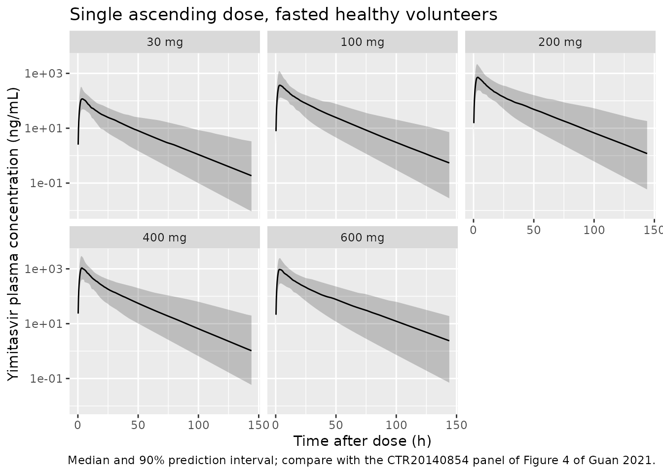
A virtual healthy-volunteer cohort of 100 subjects per dose level (30, 100, 200, 400 and 600 mg single fasted doses, sampled to 144 h as in study CTR20140854), with 25% females and ALT drawn log-normally around the healthy volunteer median of 13 IU/L (Table 2).
set.seed(20210128)
rxode2::rxSetSeed(20210128)
n_per <- 100
doses <- c(30, 100, 200, 400, 600)
obs_times <- sort(unique(c(seq(0, 12, by = 0.25), seq(13, 48, by = 1), seq(50, 144, by = 2))))

make_arm <- function(dose, id_offset) {
  subj <- tibble::tibble(
    id = id_offset + seq_len(n_per),
    SEXF = rbinom(n_per, 1, 0.25),
    ALT = pmin(pmax(exp(rnorm(n_per, log(13), 0.4)), 5), 34),
    HCV_POS = 0, FED_HIGHFAT = 0, MEAL_PREDOSE_4H = 0,
    DOSE = dose, dose_mg = dose, treatment = paste0(dose, " mg")
  )
  bind_rows(
    subj |> mutate(time = 0, evid = 1L, amt = dose, cmt = "depot", rate = -2),
    tidyr::crossing(subj, time = obs_times) |> mutate(evid = 0L, amt = 0, cmt = "central", rate = 0)
  )
}
# rxode2 drops a covariate column named DOSE that precedes `amt` ("required
# for solving: DOSE"), so the event columns go first.
ev_sad <- bind_rows(lapply(seq_along(doses), \(i) make_arm(doses[i], (i - 1L) * n_per))) |>
  relocate(id, time, evid, amt, cmt, rate) |>
  arrange(id, time, desc(evid))
stopifnot(!anyDuplicated(unique(ev_sad[, c("id", "time", "evid")])))

sim_sad <- rxode2::rxSolve(mod, ev_sad, keep = c("treatment", "dose_mg"), returnType = "data.frame")
#> ℹ parameter labels from comments will be replaced by 'label()'
sim_sad$treatment <- factor(sim_sad$treatment, levels = paste0(doses, " mg"))
sim_sad |>
  filter(time > 0) |>
  group_by(treatment, time) |>
  summarise(
    Q05 = quantile(Cc, 0.05), Q50 = median(Cc), Q95 = quantile(Cc, 0.95),
    .groups = "drop"
  ) |>
  ggplot(aes(time, Q50)) +
  geom_ribbon(aes(ymin = Q05, ymax = Q95), alpha = 0.25) +
  geom_line() +
  facet_wrap(~treatment) +
  scale_y_log10() +
  labs(
    x = "Time after dose (h)", y = "Yimitasvir plasma concentration (ng/mL)",
    title = "Single ascending dose, fasted healthy volunteers",
    caption = "Median and 90% prediction interval; compare with the CTR20140854 panel of Figure 4 of Guan 2021."
  )
PKNCA validation
sim_nca <- sim_sad |>
  filter(!is.na(Cc)) |>
  select(id, time, Cc, treatment)
dose_df <- ev_sad |>
  filter(evid == 1) |>
  select(id, time, amt, treatment)

conc_obj <- PKNCA::PKNCAconc(sim_nca, Cc ~ time | treatment + id)
dose_obj <- PKNCA::PKNCAdose(dose_df, amt ~ time | treatment + id)
intervals <- data.frame(
  start = 0, end = Inf,
  cmax = TRUE, tmax = TRUE, aucinf.obs = TRUE, half.life = TRUE
)
nca_res <- PKNCA::pk.nca(PKNCA::PKNCAdata(conc_obj, dose_obj, intervals = intervals))
nca_wide <- as.data.frame(nca_res$result) |>
  select(treatment, id, PPTESTCD, PPORRES) |>
  tidyr::pivot_wider(names_from = PPTESTCD, values_from = PPORRES)

nca_wide |>
  group_by(treatment) |>
  summarise(
    Cmax = median(cmax), Tmax = median(tmax),
    AUCinf = median(aucinf.obs) / 1000, t_half = median(half.life),
    .groups = "drop"
  ) |>
  arrange(as.numeric(sub(" mg", "", treatment))) |>
  mutate(across(where(is.numeric), \(x) signif(x, 3))) |>
  dplyr::rename(
    "Dose" = treatment, "Cmax (ng/mL)" = Cmax, "Tmax (h)" = Tmax,
    "AUC0-inf (ug*h/mL)" = AUCinf, "t1/2 (h)" = t_half
  ) |>
knitr::kable(caption = "Simulated single-dose NCA (medians of 100 subjects per dose).")| Dose | Cmax (ng/mL) | Tmax (h) | AUC0-inf (ug*h/mL) | t1/2 (h) |
|---|---|---|---|---|
| 30 mg | 117 | 3.5 | 2.16 | 17.4 |
| 100 mg | 371 | 3.5 | 7.31 | 17.1 |
| 200 mg | 717 | 3.5 | 11.90 | 17.2 |
| 400 mg | 1090 | 3.5 | 17.60 | 16.4 |
| 600 mg | 955 | 3.5 | 17.90 | 18.2 |
The dose-dependent bioavailability flattens exposure above 400 mg: the simulated AUC0-inf at 600 mg is close to that at 400 mg, in line with the single ascending dose observation quoted in the Discussion of Guan 2021 (“Similar exposures were found between 400 and 600 mg groups”).
Guan 2021 does not print NCA values, so there is no published table
to compare against. Instead, each subject’s AUC0-inf must satisfy
AUC0-inf x CL/F = F(dose) x Dose with that subject’s own
clearance and relative bioavailability, which checks the dose-dependent
F of Eq. 3, the food/sex/ALT multipliers and the unit conversion
together:
indiv <- sim_sad |>
  group_by(id) |>
  summarise(cl = first(cl), fdepot = first(fdepot), DOSE = first(dose_mg), .groups = "drop")
mb <- nca_wide |>
  mutate(id = as.integer(id)) |>
  inner_join(indiv, by = "id") |>
  mutate(ratio = (aucinf.obs / 1000) * cl / (fdepot * DOSE))

stopifnot(
  nrow(mb) == length(doses) * n_per,
  abs(median(mb$ratio) - 1) < 0.02,
  quantile(abs(mb$ratio - 1), 0.9) < 0.05
)

# Less than dose-proportional exposure: dose-normalised AUC falls with dose
# exactly as Eq. 3 predicts, relative to 100 mg.
dn <- mb |>
  group_by(DOSE) |>
  summarise(dn_auc = median(aucinf.obs * cl / DOSE), .groups = "drop") |>
  mutate(rel = dn_auc / dn_auc[DOSE == 100], expected = ifelse(DOSE <= 100, 1, 1 - 0.129 * (DOSE - 100) / 100))
stopifnot(all(abs(dn$rel / dn$expected - 1) < 0.03))
Assumptions and deviations
- IIV scale. Table 3 does not say whether the random-effect entries are variances or standard deviations. The maintainers read 0.485 and 0.736 as standard deviations and 0.565 as the CL/F-V1/F correlation (covariance 0.2017), because that reading alone reproduces the 5th percentile of the Figure 5 AUCss range (see ‘IIV scale’), matches the Results’ description of the IIV as 48.5% and 73.6%, and keeps 0.565 a valid entry of the matrix. The residual error 0.305 is taken as the proportional standard deviation (Phoenix NLME reports residual error as a standard deviation).
- 600 mg relative bioavailability. The Results print relative bioavailabilities of 87.1%, 61.3% and 45.5% for 200, 400 and 600 mg. Eq. 3 with the fixed Alpha = 0.129 gives 87.1%, 61.3% and 35.5%; the two lower doses match exactly, so 45.5% is treated as a typographical error and Eq. 3 is packaged as printed. Eq. 3 is linear without a floor, so F reaches zero at 875 mg; the model is only supported over the studied 30-600 mg range.
-
Food status encoding. The paper’s three-level food
status is decomposed into two indicators:
FED_HIGHFAT(level 2, high-fat meal in the food-effect crossover) andMEAL_PREDOSE_4H(level 1, the phase 1b evening dose at least 4 h after dinner). Level 0, the reference, is a dose after an overnight fast of at least 10 h. The paper also coded the phase 2 sparse-sampling patients, who dosed at least 2 h before or after a meal, as level 0 (Discussion); to reproduce the paper’s coding set both indicators to 0 for such patients. -
Disease status. The patient effect on Td is carried
by
HCV_POS(1 = chronic HCV genotype 1 patient, 0 = healthy volunteer). -
Dose covariate. Eq. 3 depends on the administered
dose, supplied as the
DOSEcolumn (mg per administration); it must equal the dose record’samt. Place theDOSEcolumn afteramtin the event table: rxode2 (checked with 5.1.8) does not pass aDOSEcolumn that precedesamtto the model and stops with “required for solving: DOSE”. Dose records needrate = -2so that the modelled zero-order duration is used. - ALT. Baseline ALT in IU/L (numerically equal to U/L), normalised by the population median 31.6 IU/L. The small differences (up to 0.43 percentage points) between the simulated and printed ALT bars of Figure 5 are consistent with the rounded 5th and 95th percentile ALT values (9 and 153 IU/L) printed on the figure.
- Virtual cohort. The single-dose cohort’s sex split and ALT distribution follow the healthy-volunteer column of Table 2; individual covariates of the original subjects are not available.
- No erratum or correction notice for this article was found as of 2026-09-27.