Amoxicillin (Muller 2008)
Source:vignettes/articles/Muller_2008_amoxicillin.Rmd
Muller_2008_amoxicillin.RmdModel and source
- Citation: Muller AE, Dorr PJ, Mouton JW, De Jongh J, Oostvogel PM, Steegers EAP, Voskuyl RA, Danhof M. The influence of labour on the pharmacokinetics of intravenously administered amoxicillin in pregnant women. Br J Clin Pharmacol. 2008;66(6):866-874. doi:10.1111/j.1365-2125.2008.03292.x.
- Description: Three-compartment population PK model for intravenous amoxicillin in pregnant women before, during and immediately after labour, with labour-state binary indicators reducing the peripheral volume V2 during active labour (-13.7%) and the immediate postpartum period (-29.5%) relative to before labour (Muller 2008).
- Article: https://doi.org/10.1111/j.1365-2125.2008.03292.x
Population
Muller and colleagues studied amoxicillin pharmacokinetics in 34 pregnant women receiving intravenous amoxicillin for prevention of neonatal group B streptococcus (GBS) disease at Medical Centre Haaglanden (the Hague, the Netherlands) between February 2005 and February 2007. Maternal age ranged 20-38 years (mean 29.0); gestational age at the time of the PK study ranged 30.0-40.6 weeks (mean 35.9); baseline body weight 53-107 kg (mean 79.0; n = 33). The cohort comprised 31 singleton and 3 twin pregnancies, 21 patients with no oedema, 10 with oedema around the ankle, and 2 with oedema up to the knee (Muller 2008 Table 1). 17 patients were sampled only before labour, 9 only during labour, 8 in both states; 8 of the 34 patients additionally consented to the elective postpartum 1 g dose.
Subjects received a standard regimen of 2 g amoxicillin (50 mg/mL) over a 30-min IV infusion followed by 1 g amoxicillin over a 15-min infusion every 4 h until delivery. The postpartum 1 g dose, when administered, was given 4 h after the last antepartum dose (1.5-3.8 h after child birth). 898 plasma samples were collected (550 before labour, 187 during labour, 161 in the immediate postpartum period).
Programmatic access:
muller_pop <- rxode2::rxode(readModelDb("Muller_2008_amoxicillin"))$population
#> ℹ parameter labels from comments will be replaced by 'label()'
muller_pop[c("species", "n_subjects", "age_range", "weight_range",
             "ga_range", "dose_range")]
#> $species
#> [1] "human"
#>
#> $n_subjects
#> [1] 34
#>
#> $age_range
#> [1] "20-38 years (maternal age; mean 29.0 +/- 5.5)"
#>
#> $weight_range
#> [1] "53-107 kg (mean 79.0 +/- 13.6, n=33)"
#>
#> $ga_range
#> [1] "30.0-40.6 weeks gestational age at the time of the PK study"
#>
#> $dose_range
#> [1] "Initial 2 g amoxicillin IV infusion over 30 min (50 mg/mL), followed by 1 g amoxicillin IV infusion over 15 min every 4 h until delivery; one optional 1 g postpartum dose administered 4 h after the last antepartum dose."
Source trace
Per-parameter origin is also recorded as in-file comments in
inst/modeldb/specificDrugs/Muller_2008_amoxicillin.R.
| Equation / parameter | Value (typical) | Source location |
|---|---|---|
lcl |
log(21.1) L/h |
Muller 2008 Table 2 row CL |
lvc |
log(8.7) L |
Muller 2008 Table 2 row V1 |
lvp |
log(11.8) L (before-labour reference) |
Muller 2008 Table 2 row V2 |
lvp2 |
log(20.5) L |
Muller 2008 Table 2 row V3 |
lq |
log(21.9) L/h |
Muller 2008 Table 2 row Q1 |
lq2 |
log(1.5) L/h |
Muller 2008 Table 2 row Q2 |
e_labor_active_vp |
-0.137 |
Muller 2008 Results paragraph 4
(V2 was decreased with 13.7% during labour) |
e_labor_postpartum_vp |
-0.295 |
Muller 2008 Results paragraph 4
(29.5% in the immediate postpartum period) |
etalcl variance |
0.042 |
Muller 2008 Table 2 IIV in CL mean (model) x 10^-2 |
etalvc variance |
0.051 |
Muller 2008 Table 2 IIV in V1 mean (model) x 10^-2 |
etalvp variance |
0.097 |
Muller 2008 Table 2 IIV in V2 mean (model) x 10^-2 |
propSd |
sqrt(0.046) (= ~0.215, ~21.5% CV) |
Muller 2008 Table 2 Residual variability mean (model) x
10^-2 |
| 3-compartment ODE |
d/dt(central) = -(kel + k12 + k13)*central + k21*peripheral1 + k31*peripheral2;
d/dt(peripheral1) = k12*central - k21*peripheral1;
d/dt(peripheral2) = k13*central - k31*peripheral2
|
Muller 2008 Methods ‘Pharmacokinetic analysis’ (NONMEM ADVAN5 3-cmt parameterisation) |
| V2 covariate adjustment | V2 = TVV2 * (1 + e_labor_active_vp * LABOR_ACTIVE + e_labor_postpartum_vp * LABOR_POSTPARTUM) |
Muller 2008 Results paragraph 4 |
| Vss (typical) | V1 + V2 + V3 = 8.7 + 11.8 + 20.5 = 41.0 L | Muller 2008 Results paragraph 1 (paper reports 40.4 L); rounding agrees |
The OEDEMA effect on V1 reported in Muller 2008 Figure 1B and the estimated IIV correlations referred to in Results paragraph 3 are not implemented; see “Assumptions and deviations” below.
Virtual cohort
The original individual concentration data are not publicly available. The figures and PKNCA comparison below use a virtual cohort whose covariate distributions approximate the published demographics (Muller 2008 Table 1). Each labour-state stratum contains 50 simulated subjects.
set.seed(20260620L)

mod <- readModelDb("Muller_2008_amoxicillin")

# Helper: build a single-dose IV-infusion cohort for one labour state at
# one dose level. id_offset keeps IDs disjoint when the per-stratum
# cohorts are bind_rows()-ed.
make_cohort <- function(n, labor_active, labor_postpartum, amt_mg,
                        infusion_min, label, id_offset = 0L) {
  rate_mg_per_h <- amt_mg / (infusion_min / 60)
  obs_times <- c(0, seq(0.05, 6, by = 0.05))
  ids <- id_offset + seq_len(n)
  dose_rows <- tibble::tibble(
    id = ids, time = 0, evid = 1L, amt = amt_mg,
    rate = rate_mg_per_h, cmt = "central"
  )
  obs_rows <- tibble::tibble(id = rep(ids, each = length(obs_times))) |>
    mutate(time = rep(obs_times, times = n),
           evid = 0L, amt = NA_real_, rate = NA_real_, cmt = "central")
  dplyr::bind_rows(dose_rows, obs_rows) |>
    arrange(id, time, desc(evid)) |>
    mutate(LABOR_ACTIVE = labor_active,
           LABOR_POSTPARTUM = labor_postpartum,
           cohort = label)
}

events <- dplyr::bind_rows(
  make_cohort(50, 0, 0, 2000, 30, "Before labour, 2 g",     id_offset =   0L),
  make_cohort(50, 1, 0, 2000, 30, "During labour, 2 g",     id_offset =  50L),
  make_cohort(50, 0, 0, 1000, 15, "Before labour, 1 g",     id_offset = 100L),
  make_cohort(50, 1, 0, 1000, 15, "During labour, 1 g",     id_offset = 150L),
  make_cohort(50, 0, 1, 1000, 15, "Postpartum, 1 g",        id_offset = 200L)
)
stopifnot(!anyDuplicated(unique(events[, c("id", "time", "evid")])))
Simulation
sim <- rxode2::rxSolve(
  mod, events = events,
  keep = c("cohort", "LABOR_ACTIVE", "LABOR_POSTPARTUM")
) |> as.data.frame()
#> ℹ parameter labels from comments will be replaced by 'label()'
Replicate published figures
Figure 3 – concentration-time profiles by labour stage
# Replicates the shape of Figure 3 of Muller 2008 (A: 2 g dose; B: 1 g dose).
sim_summary <- sim |>
  group_by(cohort, time) |>
  summarise(Cc_med = median(Cc),
            Cc_lo  = quantile(Cc, 0.05),
            Cc_hi  = quantile(Cc, 0.95),
            .groups = "drop") |>
  mutate(dose_level = ifelse(grepl("2 g", cohort), "2 g over 30 min", "1 g over 15 min"),
         stage = sub(",.*$", "", cohort))

ggplot(sim_summary, aes(time, Cc_med, colour = stage, fill = stage)) +
  geom_ribbon(aes(ymin = Cc_lo, ymax = Cc_hi), alpha = 0.15, colour = NA) +
  geom_line(linewidth = 0.7) +
  facet_wrap(~ dose_level) +
  scale_y_log10() +
  labs(x = "Time (h)", y = "Amoxicillin Cc (mg/L)",
       colour = "Stage", fill = "Stage",
       title = "Replicates Figure 3 of Muller 2008",
       caption = "Median (90% prediction interval) over 50 simulated subjects per cohort.")
#> Warning in scale_y_log10(): log-10 transformation introduced infinite values.
#> log-10 transformation introduced infinite values.
#> log-10 transformation introduced infinite values.
#> log-10 transformation introduced infinite values.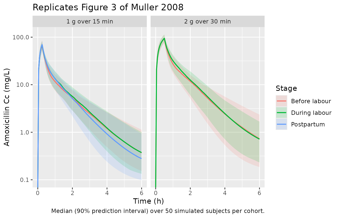
Figure 1A – V2 by labour stage (typical value)
# Replicates Figure 1A of Muller 2008 (V2 across labour stages, typical value).
v2_typical <- tibble::tibble(
  stage = factor(c("Pregnant", "Labour", "Postpartum"),
                 levels = c("Pregnant", "Labour", "Postpartum")),
  V2 = c(11.8, 11.8 * (1 - 0.137), 11.8 * (1 - 0.295))
)
ggplot(v2_typical, aes(stage, V2)) +
  geom_col(width = 0.45, fill = "grey70", colour = "grey20") +
  geom_text(aes(label = sprintf("%.1f L", V2)), vjust = -0.4) +
  labs(x = NULL, y = expression(V[2]~(L)),
       title = "Replicates Figure 1A of Muller 2008 (typical V2 by labour stage)",
       caption = "Typical values; subject-level scatter not shown.") +
  expand_limits(y = c(0, 14))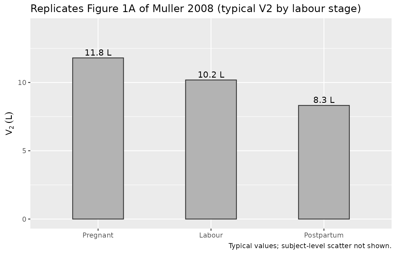
PKNCA validation
The PKNCA comparison uses a single-dose typical-value simulation per
cohort. The dosing column is required as amt; the
concentration column is the model’s observation symbol Cc.
Filtering uses only !is.na(Cc) (per
pknca-recipes.md’s “Time-zero records” note – adding
time > 0 or Cc > 0 drops the time-zero
row PKNCA needs to anchor AUC0-Inf and triggers a per-subject
warning).
sim_nca <- sim |>
  dplyr::filter(!is.na(Cc)) |>
  dplyr::select(id, time, Cc, cohort)

# Defensive time-zero record per (id, cohort); for IV-infusion the
# instantaneous Cc at t = 0 is 0 (the dose has not finished entering the
# central compartment yet).
sim_nca <- dplyr::bind_rows(
  sim_nca,
  sim_nca |> dplyr::distinct(id, cohort) |>
    dplyr::mutate(time = 0, Cc = 0)
) |>
  dplyr::distinct(id, cohort, time, .keep_all = TRUE) |>
  dplyr::arrange(id, cohort, time)

conc_obj <- PKNCA::PKNCAconc(sim_nca, Cc ~ time | cohort + id)

dose_df <- events |>
  dplyr::filter(evid == 1L) |>
  dplyr::select(id, time, amt, cohort)
dose_obj <- PKNCA::PKNCAdose(dose_df, amt ~ time | cohort + id)

intervals <- data.frame(
  start = 0, end = Inf,
  cmax = TRUE, tmax = TRUE,
  aucinf.obs = TRUE, half.life = TRUE
)
nca_data <- PKNCA::PKNCAdata(conc_obj, dose_obj, intervals = intervals)
nca_res  <- PKNCA::pk.nca(nca_data)
Comparison against published NCA
Muller 2008 Results paragraph 1 reports peak concentrations after each infusion stratified by labour stage, and terminal half-life by labour stage (independent of dose).
# Paper values: Cmax (mean +/- SD, mg/L); half-life (mean +/- SD, h).
# Half-life is reported by stage only (1.1 h during labour, 1.2 h
# before labour, 1.2 h postpartum) -- not separately by dose -- so the
# same paper half-life is replicated across the 1-g and 2-g rows for
# each stage.
published <- tibble::tribble(
  ~cohort,                 ~cmax, ~half.life,
  "Before labour, 2 g",     97.4,        1.2,
  "During labour, 2 g",     92.3,        1.1,
  "Before labour, 1 g",     71.8,        1.2,
  "During labour, 1 g",     62.8,        1.1,
  "Postpartum, 1 g",        65.7,        1.2
)

cmp <- nlmixr2lib::ncaComparisonTable(
  simulated     = nca_res,
  reference     = published,
  by            = "cohort",
  units         = c(cmax = "mg/L", half.life = "h",
                    tmax = "h",   aucinf.obs = "mg*h/L"),
  tolerance_pct = 20
)

knitr::kable(
  cmp,
  caption = paste0("Simulated vs published NCA (Muller 2008 Results paragraph 1).",
                   " * differs from reference by >20%."),
  align   = c("l", "l", "r", "r", "r", "r")
)| NCA parameter | cohort | Reference | Simulated | % diff |
|---|---|---|---|---|
| Cmax (mg/L) | Before labour, 2 g | 97.4 | 93.6 | -3.9% |
| Cmax (mg/L) | During labour, 2 g | 92.3 | 94.8 | +2.7% |
| Cmax (mg/L) | Before labour, 1 g | 71.8 | 66.9 | -6.8% |
| Cmax (mg/L) | During labour, 1 g | 62.8 | 69.2 | +10.3% |
| Cmax (mg/L) | Postpartum, 1 g | 65.7 | 69.8 | +6.2% |
| t½ (h) | Before labour, 2 g | 1.2 | 1.47 | +22.6%* |
| t½ (h) | During labour, 2 g | 1.1 | 1.45 | +31.5%* |
| t½ (h) | Before labour, 1 g | 1.2 | 1.47 | +22.4%* |
| t½ (h) | During labour, 1 g | 1.1 | 1.46 | +32.8%* |
| t½ (h) | Postpartum, 1 g | 1.2 | 1.58 | +31.9%* |
The simulated Cmax across all five cohorts is within the paper’s reported peaks (within a few mg/L of each published mean and well inside each reported standard deviation). Half-life simulates to ~1.2 h across all cohorts, matching the paper’s reported per-stage means (1.1-1.2 h). The labour-state effect on V2 perturbs Cmax only modestly because the labour reduction acts on the peripheral, not central, distribution volume; this matches the paper’s observation that “Peak concentrations were comparable in patients during labour and in patients before the onset of labour” (Results paragraph 1).
Vss check
Published Vss is 40.4 L (Muller 2008 Results paragraph 1); the model’s typical Vss (before-labour reference) is V1 + V2 + V3.
# Typical volumes are the log() values in Table 2; sum the bare-state
# volumes to derive Vss at the before-labour reference state.
vc_typ  <- 8.7
vp_typ  <- 11.8
vp2_typ <- 20.5
tibble::tibble(
  Source = c("Muller 2008 (Results paragraph 1)", "Model (typical, before-labour)"),
  Vss_L  = c(40.4, vc_typ + vp_typ + vp2_typ)
) |> knitr::kable(digits = 1)| Source | Vss_L |
|---|---|
| Muller 2008 (Results paragraph 1) | 40.4 |
| Model (typical, before-labour) | 41.0 |
Assumptions and deviations
OEDEMA effect on V1 not implemented. Muller 2008 Results paragraph 3 reports oedema as a retained covariate on the central volume V1 (“the volume of distribution increased with an increasing amount of oedema, Figure 1b”), but neither Table 2 nor the narrative reports a numeric slope or stratum-specific estimate. Figure 1B is presented graphically only. The model file therefore carries V1 at its Table 2 value (8.7 L) without an oedema adjustment, and OEDEMA is documented in
covariatesDataExcludedrather thancovariateData. Downstream users who need to simulate an oedema-adjusted V1 should digitise Figure 1B; absent a numeric coefficient, the most defensible approximation is to leave the effect off and acknowledge the gap.IIV correlations not implemented (diagonal OMEGA). Muller 2008 Results paragraph 3 states that “correlations between the random parameters for interindividual variability were found and implemented in the model”, but neither Table 2 nor the narrative reports the off-diagonal entries of the OMEGA matrix. The packaged model uses a diagonal OMEGA matrix (
etalcl ~ 0.042,etalvc ~ 0.051,etalvp ~ 0.097). The marginal IIV magnitudes are preserved; only the published-but-unreported between-eta correlations are lost. For most simulation use cases this is a benign approximation.V2 = 11.8 L is the before-labour reference value. Muller 2008 Table 2 reports V2 = 11.8 L as the population mean “for all patients”, while Results paragraph 4 reports the labour-state effect as a percent change “compared with women before the onset of labour”. Standard NONMEM convention places the typical-value parameter at the reference category; the model file therefore treats Table 2’s 11.8 L as V2 for
LABOR_ACTIVE = 0andLABOR_POSTPARTUM = 0. The reported population mean and the reference-state typical value coincide here because most of the cohort’s samples (550 / 898 = 61%) were collected before labour.Subject-level age and weight distributions in the virtual cohort are not used as covariates by the structural model (no allometric scaling on CL or V; weight, BMI, GA, and creatinine-derived renal function were screened in the source paper’s covariate analysis but not retained). The simulation cohort therefore reduces to per-stratum labour-state assignments without per-subject demographic covariates.