Unbound and total mycophenolic acid with MPAG (Sheng 2020)
Source:vignettes/articles/Sheng_2020_mycophenolic_acid.Rmd
Sheng_2020_mycophenolic_acid.RmdModel and source
- Citation: Sheng C, Zhao Q, Niu W, Qiu X, Zhang M, Jiao Z. Effect of Protein Binding on Exposure of Unbound and Total Mycophenolic Acid: A Population Pharmacokinetic Analysis in Chinese Adult Kidney Transplant Recipients. Front Pharmacol. 2020;11:340. doi:10.3389/fphar.2020.00340.
- Description: Population PK model of unbound and total mycophenolic acid (uMPA, tMPA) and its 7-O-glucuronide metabolite (MPAG) in Chinese adult kidney transplant recipients co-treated with cyclosporine and given oral mycophenolate mofetil (MMF) (Sheng 2020). Five compartments (Figure 1): a gut depot with first-order absorption and a lag time, a two-compartment disposition of UNBOUND MPA (central + peripheral1), a one-compartment disposition of unbound MPAG (central_mpag), and a gallbladder (gallbladder_mpag) giving intermittent enterohepatic circulation. 87 percent of uMPA elimination forms MPAG (fixed); the rest is eliminated directly. Total MPA is linked to unbound MPA by a linear protein-binding constant, tMPA = uMPA * (1 + kB), with kB proportional to serum albumin; total MPAG = unbound MPAG / 0.18 (fixed unbound fraction). The gallbladder fills from central_mpag at a rate set by the estimated fraction of MPAG recycled and empties into the gut (where MPAG is assumed fully deconjugated to MPA and reabsorbed) at a fixed first-order rate during a 0.5 h window after each meal. Meal gates are read against time after the most recent dose (tad()) at 4 and 10 h, the study-1 schedule. Covariates: body weight on Q/F of uMPA, serum albumin on kB, glomerular filtration rate (CKD-EPI, mL/min) on CL/F of uMPAG. Dose in mg MMF; the model works internally in umol and reports concentrations in mg/L.
- Article: https://doi.org/10.3389/fphar.2020.00340 (open access)
The model describes three measured analytes after oral mycophenolate
mofetil (MMF): unbound mycophenolic acid (uMPA, output
Cunbound), total MPA (tMPA, output Cc) and
total 7-O-mycophenolic acid glucuronide (tMPAG, output
Cc_mpag). All disposition parameters refer to UNBOUND
concentrations; the totals are reconstructed algebraically,
tMPA = uMPA * (1 + kB) (Eq 1) and
tMPAG = uMPAG / 0.18.
Population
Fifty-eight Chinese adult first-time kidney transplant recipients on MMF, cyclosporine and corticosteroids, pooled from an early post-transplant study (Jiao 2007; 20 patients, 27 full 12 h profiles, mostly within 3 months of transplant) and a stable-phase bioequivalence study (Geng 2012; 38 patients, 38 profiles, mostly beyond 3 months). Table 1 of Sheng 2020 gives (median (range), study 1 / study 2): age 36 (19-61) / 38 (18-62) years; body weight 55 (40-71) / 65 (42-82.5) kg; serum albumin 31 (20-43) / 44.9 (32.3-50) g/L; CKD-EPI GFR 76.1 (11.2-123.8) / 74.4 (45.1-102.3) mL/min; MMF 1500 / 1000 mg/day; 13 of 58 patients (22%) female. 740 uMPA, 741 tMPA and 734 tMPAG concentrations were analysed.
The same information is available programmatically via
rxode2::rxode(readModelDb("Sheng_2020_mycophenolic_acid"))$population.
Source trace
| Equation / parameter | Value | Source location |
|---|---|---|
| Structure: gut, uMPA central + peripheral, uMPAG central, gallbladder | – | Figure 1; Results ‘Model Development’ |
lka |
1.35 1/h | Table 2 |
ltlag |
0.447 h | Table 2 |
lcl (CLuMPA/F) |
851 L/h | Table 2 |
lvc (VCuMPA/F) |
718 L | Table 2 |
lq (QuMPA/F at 70 kg) |
857 L/h | Table 2, footnote c |
e_wt_q |
2.11 | Table 2, footnote c |
lvp (VPuMPA/F) |
34,300 L (fixed) | Results; Table 3 |
fm (MPA to MPAG) |
0.87 (fixed) | Methods assumption 2; Figure 1 (k24 87%, k20 13%) |
lkns (kB at ALB 40 g/L) |
53.4 | Table 2, footnote d; Eq 1 |
e_alb_kns |
1 (fixed) | Results; footnote d |
lcl_mpag (CLuMPAG/F at GFR 80 mL/min) |
5.71 L/h | Table 2, footnote e |
e_crcl_cl_mpag |
0.865 | Table 2, footnote e |
lvc_mpag (VCuMPAG/F) |
29.9 L | Table 2 |
fu_mpag |
0.18 (fixed) | Methods |
lehcp (%EHC / 100) |
0.0553 | Table 2; Eq 4 %EHC = kGG / (kGG + ke0) * 100
|
lkehc (kGB) |
3.708 1/h (fixed) | Methods; Figure 1 |
dge (DGB) |
0.5 h (fixed) | Methods; Figure 1 |
tmeal1, tmeal2
|
4, 10 h after dose (fixed) | Methods, ‘Study Design and Patients’ (study 1) |
| BSV (omega^2 = (CV/100)^2) | CL 51.0%, Q 45.5%, VC 80.0%, ka 46.5%, Tlag 107.7%, kB 10% (fixed), CLuMPAG 31.8%, VCuMPAG 48.4% (r = 0.574), %EHC 61.6% | Table 2; Results (kB variance 0.01) |
expSd, expSd_Cunbound,
expSd_mpag
|
0.459, 0.470, 0.220 | Table 2 (exponential RUV) |
fu = 1 / (1 + kB) |
derived | Eq 2 |
| MW MMF / MPA / MPAG | 433.498 / 320.339 / 496.462 g/mol | Methods, ‘Software and Model Selection Criteria’ |
Deterministic checks
The typical-value solves below switch off all random effects
(omega = NA, sigma = NA), so the comparisons are exact and
use tight bounds.
mod <- rxode2::rxode(readModelDb("Sheng_2020_mycophenolic_acid"))
#> ℹ parameter labels from comments will be replaced by 'label()'
stopifnot(identical(
  mod$state,
  c("depot", "central", "peripheral1", "central_mpag", "gallbladder_mpag")
))

n_dose <- 60
tau    <- 12
t_ss   <- (n_dose - 1) * tau
# Paper sampling schedule (study 1) within the steady-state interval.
samp   <- c(0, 0.5, 1, 1.5, 2, 3, 4, 6, 8, 10, 12)

make_events <- function(ids, obs_times, dvids = 1L) {
  dose <- data.frame(
    time = seq(0, by = tau, length.out = n_dose), amt = 750, evid = 1L,
    cmt = "depot", dvid = NA_integer_
  )
  obs <- expand.grid(time = obs_times, dvid = dvids)
  obs <- data.frame(time = obs$time, amt = 0, evid = 0L, cmt = NA_character_, dvid = obs$dvid)
  one <- dplyr::bind_rows(dose, obs)
  dplyr::bind_rows(lapply(ids, function(i) dplyr::mutate(one, id = i))) |>
    dplyr::arrange(id, time, evid)
}

solve_typical <- function(ALB, CRCL, WT = 70, obs_times = t_ss + seq(0, 12, by = 0.05)) {
  ev <- make_events(1L, obs_times)
  ev$ALB <- ALB
  ev$CRCL <- CRCL
  ev$WT <- WT
  rxode2::rxSolve(mod, ev,
    omega = NA, sigma = NA, returnType = "data.frame",
    useLinCmt = FALSE
  )
}

trap <- function(x, y) sum(diff(x) * (head(y, -1) + tail(y, -1)) / 2)
Unbound fraction and the total-scale parameters
Eq 2 gives FUMPA = 1 / (1 + kB). Table 2 footnote f
lists the total-scale parameters obtained by multiplying the unbound
ones by the typical unbound fraction at 40 g/L albumin, and Results
quote the unbound fraction at 40 and 20 g/L.
fu40 <- solve_typical(40, 90)$fu[1]
fu20 <- solve_typical(20, 90)$fu[1]
tot <- tibble::tribble(
  ~quantity,          ~unbound, ~published_total,
  "CL/F of MPA (L/h)",  851,      15.66,
  "Q/F of MPA (L/h)",   857,      15.77,
  "Vc/F of MPA (L)",    718,      13.21,
  "Vp/F of MPA (L)",    34300,    631.12,
  "CL/F of MPAG (L/h)", 5.71,     1.03,
  "Vc/F of MPAG (L)",   29.9,     5.38
) |>
  dplyr::mutate(
    fu = c(rep(fu40, 4), rep(0.18, 2)),
    model_total = unbound * fu,
    pct_diff = 100 * (model_total / published_total - 1)
  )
knitr::kable(
  dplyr::rename(tot,
    "Quantity" = quantity, "Unbound value" = unbound,
    "Published total (Table 2)" = published_total, "Unbound fraction" = fu,
    "Model total" = model_total, "Difference (%)" = pct_diff
  ),
  digits = 4,
  caption = "Total-scale parameters: model (unbound value times unbound fraction) vs Table 2 footnote f."
)| Quantity | Unbound value | Published total (Table 2) | Unbound fraction | Model total | Difference (%) |
|---|---|---|---|---|---|
| CL/F of MPA (L/h) | 851.00 | 15.66 | 0.0184 | 15.6434 | -0.1061 |
| Q/F of MPA (L/h) | 857.00 | 15.77 | 0.0184 | 15.7537 | -0.1035 |
| Vc/F of MPA (L) | 718.00 | 13.21 | 0.0184 | 13.1985 | -0.0868 |
| Vp/F of MPA (L) | 34300.00 | 631.12 | 0.0184 | 630.5147 | -0.0959 |
| CL/F of MPAG (L/h) | 5.71 | 1.03 | 0.1800 | 1.0278 | -0.2136 |
| Vc/F of MPAG (L) | 29.90 | 5.38 | 0.1800 | 5.3820 | 0.0372 |
Steady-state mass balance and unbound invariance
At steady state the dose-interval AUC of uMPA equals the MPA input
rate over the unbound clearance. Recycling returns a fraction
fm * ehcp of MPA elimination to the gut, so
AUCu,tau = Dose_MPA / (CL * (1 - fm * ehcp)), independent
of albumin and of GFR (the paper’s central clinical claim). The
total-MPA AUC scales with 1 + kB.
dose_mpa <- 750 * 320.339 / 433.498 # mg MPA per MMF dose
auc_u_theory <- dose_mpa / (851 * (1 - 0.87 * 0.0553))
grid <- expand.grid(ALB = c(20, 40), CRCL = c(15, 90))
ss <- dplyr::bind_rows(lapply(seq_len(nrow(grid)), function(i) {
  s <- solve_typical(grid$ALB[i], grid$CRCL[i])
  data.frame(
    ALB = grid$ALB[i], CRCL = grid$CRCL[i],
    auc_u = trap(s$time, s$Cunbound), auc_t = trap(s$time, s$Cc),
    auc_g = trap(s$time, s$Cc_mpag)
  )
}))
knitr::kable(
  dplyr::rename(ss,
    "Albumin (g/L)" = ALB, "GFR (mL/min)" = CRCL,
    "uMPA AUCtau (mg*h/L)" = auc_u, "tMPA AUCtau (mg*h/L)" = auc_t,
    "tMPAG AUCtau (mg*h/L)" = auc_g
  ),
  digits = 3,
  caption = "Typical-value steady-state AUC over one 12 h interval (750 mg MMF every 12 h, 70 kg)."
)| Albumin (g/L) | GFR (mL/min) | uMPA AUCtau (mg*h/L) | tMPA AUCtau (mg*h/L) | tMPAG AUCtau (mg*h/L) |
|---|---|---|---|---|
| 20 | 15 | 0.684 | 18.946 | 3069.552 |
| 40 | 15 | 0.684 | 37.208 | 3069.552 |
| 20 | 90 | 0.684 | 18.946 | 651.613 |
| 40 | 90 | 0.684 | 37.208 | 651.613 |
c(theory_auc_u = auc_u_theory)
#> theory_auc_u
#>    0.6841764
stopifnot(
  all(abs(ss$auc_u / auc_u_theory - 1) < 0.005),
  all(abs(ss$auc_t / (ss$auc_u * (1 + 53.4 * ss$ALB / 40)) - 1) < 1e-6),
  # Unbound exposure ignores albumin exactly (same CRCL, different ALB).
  abs(ss$auc_u[1] / ss$auc_u[2] - 1) < 1e-8
)
Covariate effects (Figure 5)
Figure 5 of Sheng 2020 shows the ratio of the AUC0-12h to the reference subject (albumin 40 g/L, GFR 90 mL/min). The published ratios below were read by the maintainers from the figure (tMPA row for albumin; tMPAG row for GFR), except the tMPA albumin-20 value, which is the ratio of the two medians quoted in Results (21.59 / 42.92).
ref <- solve_typical(40, 90)
auc_ref <- c(t = trap(ref$time, ref$Cc), g = trap(ref$time, ref$Cc_mpag))
fig5 <- tibble::tribble(
  ~analyte, ~ALB, ~CRCL, ~published,
  "tMPA",   20,   90,    21.59 / 42.92,
  "tMPA",   30,   90,    0.75,
  "tMPA",   50,   90,    1.24,
  "tMPAG",  40,   15,    4.6,
  "tMPAG",  40,   30,    2.5,
  "tMPAG",  40,   60,    1.42,
  "tMPAG",  40,   120,   0.78
)
fig5$model <- vapply(seq_len(nrow(fig5)), function(i) {
  s <- solve_typical(fig5$ALB[i], fig5$CRCL[i])
  if (fig5$analyte[i] == "tMPA") {
    trap(s$time, s$Cc) / auc_ref[["t"]]
  } else {
    trap(s$time, s$Cc_mpag) / auc_ref[["g"]]
  }
}, numeric(1))
fig5$pct_diff <- 100 * (fig5$model / fig5$published - 1)
knitr::kable(
  dplyr::rename(fig5,
    "Analyte" = analyte, "Albumin (g/L)" = ALB, "GFR (mL/min)" = CRCL,
    "Published ratio" = published, "Model ratio" = model, "Difference (%)" = pct_diff
  ),
  digits = 3,
  caption = "Replicates Figure 5 of Sheng 2020: AUC0-12h ratio to the reference subject."
)| Analyte | Albumin (g/L) | GFR (mL/min) | Published ratio | Model ratio | Difference (%) |
|---|---|---|---|---|---|
| tMPA | 20 | 90 | 0.503 | 0.509 | 1.225 |
| tMPA | 30 | 90 | 0.750 | 0.755 | 0.613 |
| tMPA | 50 | 90 | 1.240 | 1.245 | 0.436 |
| tMPAG | 40 | 15 | 4.600 | 4.711 | 2.407 |
| tMPAG | 40 | 30 | 2.500 | 2.586 | 3.458 |
| tMPAG | 40 | 60 | 1.420 | 1.420 | 0.007 |
| tMPAG | 40 | 120 | 0.780 | 0.780 | -0.038 |
The Results text reports that lowering GFR from 90 to 15 mL/min
raises tMPAG AUC0-12h 3.67-fold. Figure 5 of the same paper places that
ratio near 4.6, and the Table 2 exponent gives
6^0.865 = 4.71 at steady state; the model follows the table
and the figure (see Assumptions and deviations).
Virtual cohort and simulation
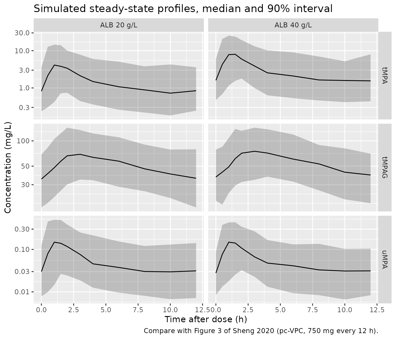
Two arms of 200 subjects each, both at the reference covariates of the paper’s simulation (70 kg, GFR 90 mL/min) with albumin 40 or 20 g/L, receive 750 mg MMF every 12 h for 30 days (the peripheral volume of 34,300 L makes the approach to steady state slow). Concentrations include between-subject and residual variability, which is how the paper computed its simulated AUC0-12h (Methods, ‘Simulation Analyses’).
rxode2::rxSetSeed(20200320)
n_arm <- 200
obs_t <- t_ss + samp
ev_st <- dplyr::bind_rows(
  make_events(seq_len(n_arm), obs_t, dvids = 1:3) |> dplyr::mutate(ALB = 40, arm = "ALB 40 g/L"),
  make_events(n_arm + seq_len(n_arm), obs_t, dvids = 1:3) |> dplyr::mutate(ALB = 20, arm = "ALB 20 g/L")
) |>
  dplyr::mutate(CRCL = 90, WT = 70)

sim <- rxode2::rxSolve(mod, ev_st,
  returnType = "data.frame", useLinCmt = FALSE,
  keep = c("arm")
)
# CMT indexes the three declared endpoints in model order.
analytes <- setNames(c("tMPA", "uMPA", "tMPAG"), c(6, 7, 8))
sim <- sim |>
  dplyr::mutate(analyte = unname(analytes[as.character(CMT)]), tad = time - t_ss)
stopifnot(!anyNA(sim$analyte))
sim |>
  dplyr::group_by(arm, analyte, tad) |>
  dplyr::summarise(
    p05 = quantile(sim, 0.05), p50 = median(sim), p95 = quantile(sim, 0.95),
    .groups = "drop"
  ) |>
  ggplot(aes(tad, p50)) +
  geom_ribbon(aes(ymin = p05, ymax = p95), alpha = 0.25) +
  geom_line() +
  scale_y_log10() +
  facet_grid(analyte ~ arm, scales = "free_y") +
  labs(
    x = "Time after dose (h)", y = "Concentration (mg/L)",
    title = "Simulated steady-state profiles, median and 90% interval",
    caption = "Compare with Figure 3 of Sheng 2020 (pc-VPC, 750 mg every 12 h)."
  )
PKNCA validation
PKNCA computes the AUC over the steady-state interval (linear trapezoidal rule on the paper’s sampling times, as in the paper) for each analyte.
conc <- sim |>
  dplyr::filter(!is.na(sim)) |>
  dplyr::select(id, time, conc = sim, analyte, arm)
dose_df <- ev_st |>
  dplyr::filter(evid == 1L) |>
  dplyr::select(id, time, amt, arm) |>
  tidyr::crossing(analyte = c("tMPA", "uMPA", "tMPAG"))

conc_obj <- PKNCA::PKNCAconc(conc, conc ~ time | arm + analyte + id, concu = "mg/L", timeu = "h")
dose_obj <- PKNCA::PKNCAdose(dose_df, amt ~ time | arm + analyte + id, doseu = "mg")
intervals <- data.frame(start = t_ss, end = t_ss + tau, auclast = TRUE, cmax = TRUE, tmax = TRUE)
nca_res <- PKNCA::pk.nca(PKNCA::PKNCAdata(conc_obj, dose_obj,
  intervals = intervals,
  options = list(auc.method = "linear")
))
summary(nca_res)
#>  Interval Start Interval End        arm analyte   N AUClast (h*mg/L)
#>             708          720 ALB 20 g/L    tMPA 200      21.7 [65.0]
#>             708          720 ALB 20 g/L   tMPAG 200       643 [32.6]
#>             708          720 ALB 20 g/L    uMPA 200     0.791 [61.3]
#>             708          720 ALB 40 g/L    tMPA 200      42.9 [52.7]
#>             708          720 ALB 40 g/L   tMPAG 200       688 [33.6]
#>             708          720 ALB 40 g/L    uMPA 200     0.765 [52.1]
#>   Cmax (mg/L)           Tmax (h)
#>   7.17 [66.3] 1.50 [0.500, 10.0]
#>   87.7 [38.3] 3.00 [0.500, 12.0]
#>  0.269 [67.7] 1.50 [0.500, 8.00]
#>   14.7 [59.4] 1.50 [0.500, 8.00]
#>   94.1 [39.7] 3.00 [0.000, 10.0]
#>  0.255 [59.5] 1.50 [0.500, 8.00]
#>
#> Caption: AUClast, Cmax: geometric mean and geometric coefficient of variation; Tmax: median and range; N: number of subjects
Comparison against published values
Results report the median simulated tMPA AUC0-12h at GFR 90 mL/min: 42.92 mgh/L at albumin 40 g/L and 21.59 mgh/L at 20 g/L.
published <- tibble::tribble(
  ~arm,         ~analyte, ~auclast,
  "ALB 40 g/L", "tMPA",   42.92,
  "ALB 20 g/L", "tMPA",   21.59
)
nca_tmpa <- nca_res
nca_tmpa$result <- dplyr::filter(nca_tmpa$result, analyte == "tMPA")
cmp <- nlmixr2lib::ncaComparisonTable(
  simulated = nca_tmpa,
  reference = published,
  by = c("arm", "analyte"),
  params = "auclast",
  units = c(auclast = "mg*h/L"),
  tolerance_pct = 20
)
knitr::kable(cmp, caption = "Simulated vs published median tMPA AUC0-12h. * differs from reference by >20%.")| NCA parameter | arm | analyte | Reference | Simulated | % diff |
|---|---|---|---|---|---|
| AUClast (mg*h/L) | ALB 40 g/L | tMPA | 42.9 | 43 | +0.1% |
| AUClast (mg*h/L) | ALB 20 g/L | tMPA | 21.6 | 21 | -2.5% |
med <- as.data.frame(nca_res$result) |>
  dplyr::filter(PPTESTCD == "auclast") |>
  dplyr::group_by(arm, analyte) |>
  dplyr::summarise(median_auc = median(PPORRES), .groups = "drop")
m40 <- med$median_auc[med$arm == "ALB 40 g/L" & med$analyte == "tMPA"]
m20 <- med$median_auc[med$arm == "ALB 20 g/L" & med$analyte == "tMPA"]
u40 <- med$median_auc[med$arm == "ALB 40 g/L" & med$analyte == "uMPA"]
u20 <- med$median_auc[med$arm == "ALB 20 g/L" & med$analyte == "uMPA"]
stopifnot(
  # Centre of the cohort, not its extremes.
  abs(m40 / 42.92 - 1) < 0.15,
  abs(m20 / 21.59 - 1) < 0.15,
  # Results: uMPA exposure 'almost unchanged (< 5%)' between ALB 40 and 20.
  abs(u20 / u40 - 1) < 0.15
)
The published medians are reproduced only when residual error is included in the simulated concentrations. The typical-value steady-state tMPA AUC is 37.2 mgh/L (deterministic table above). Lognormal residual error with SD 0.459 raises the median trapezoidal AUC of the noisy profiles by roughly 10-15%, which closes the gap to 42.92 mgh/L. The paper’s simulated AUC0-12h therefore included residual variability, and a comparison against the typical value alone would look about 13% low.
Assumptions and deviations
-
Meal times. Methods state that meals followed the 4
and 10 h samples in study 1 and the 3 and 9 h samples in study 2; the
Discussion says meal time “was set at 10 (study 1) and 9 (study 2) h
postdosing”. The model gates gallbladder emptying at 4 and 10 h after
each dose (study-1 schedule, both meals), read against
tad()so the gate recurs after every dose. Because the gallbladder has no exit other than emptying, the steady-state exposure of all three analytes is the same whichever meal schedule is used; only the timing of the secondary peaks changes. Overridetmeal1/tmeal2for study 2 or other schedules. -
Gallbladder emptying fraction. Methods state that
the 0.5 h duration ensures that over 90% of the gallbladder content is
released per trigger; with kGB = 3.708 1/h the released fraction is
1 - exp(-3.708 * 0.5)= 84%. The printed values are kept. -
kB units. Table 2 prints kB with unit 1/h, but in
Eq 1 (
CtMPA = CuMPA + kB * CuMPA) it is a dimensionless bound:unbound ratio;1 / (1 + 53.4)reproduces the reported unbound fraction of 1.84%. It is carried as the registered linear protein-binding constantkns. -
Variance scale. Table 2 %CV values are taken as
100 * sqrt(omega^2): the kB entry “10.0 FIXED” corresponds to the variance of 0.01 stated in Results. The residual %CV values are taken as log-scale SDs of the exponential error model. - Residual correlation not encoded. The final model estimated a correlation of 0.512 between the uMPA and tMPA residuals (L2 / SIGMA BLOCK). nlmixr2 residual-error models are independent per endpoint, so the three residual errors are simulated independently.
-
MPAG endpoint. The paper fitted uMPAG, derived as
0.18 times the measured tMPAG. The model reports tMPAG
(
Cc_mpag) with the uMPAG residual SD; a multiplicative constant does not change a log-scale residual. The unbound MPAG concentration is available asCunbound_mpag. - GFR 15 mL/min tMPAG ratio. The Results text quotes a 3.67-fold (95% CI 3.13-4.30) increase in tMPAG AUC0-12h from GFR 90 to 15 mL/min. Figure 5 and the Table 2 exponent (0.865, reference 80 mL/min) both give about 4.6-4.7. The model follows Table 2.
-
GFR units and reference. GFR is the CKD-EPI
estimate, labelled “mL/min” in the source, supplied here in the
CRCLcolumn. The CLuMPAG/F reference is 80 mL/min (Table 2 footnote e), not the 90 mL/min reference subject used in Table 3 and the simulations. - Molar bookkeeping. The source modelled in molar units. The model takes MMF doses in mg, converts to umol of MPA on absorption (1:1 hydrolysis), forms MPAG 1:1 in umol, and re-expresses the recycled MPAG as MMF-mass equivalents when it returns to the gut depot, so that recycled and dosed drug share the same absorption rate and lag.
-
%EHC.
%EHCcarries exponential between-subject variability as printed; a draw above 100% (more than 4.7 SD above the mean) would make the biliary rate negative, which does not occur at practical cohort sizes. -
Covariates not retained (sex, age, hemoglobin,
cyclosporine dose, antacids and others) are listed in
covariatesDataExcluded.