Pembrolizumab exposure-response in NSCLC (Chatterjee 2016)
Source:vignettes/articles/Chatterjee_2016_pembrolizumab.Rmd
Chatterjee_2016_pembrolizumab.RmdModel and source
- Citation: Chatterjee M, Turner DC, Felip E, Lena H, Cappuzzo F, Horn L, Garon EB, Hui R, Arkenau H-T, Gubens MA, Hellmann MD, Dong D, Li C, Mayawala K, Freshwater T, Ahamadi M, Stone J, Lubiniecki GM, Zhang J, Im E, De Alwis DP, Kondic AG, Flotten O. Systematic evaluation of pembrolizumab dosing in patients with advanced non-small-cell lung cancer. Ann Oncol. 2016;27(7):1291-1298. doi:10.1093/annonc/mdw174. PMID: 27117531. Structural equation and exposure-effect equation from the main-article Methods (‘tumor size NLME model structure’ and ‘exposure-efficacy analysis’); all final parameter values from supplementary Table S6; covariate parameterization from the Supplementary Methods (‘Handling of Covariates’).
- Description: Exposure-response tumor-size (sum of longest diameters, SLD) model for pembrolizumab in previously treated and treatment-naive advanced non-small-cell lung cancer (NSCLC), developed by Chatterjee et al. (Merck) on the KEYNOTE-001 NSCLC expansion cohorts (n = 496 with both tumor-size and pharmacokinetic data at 2 mg/kg Q3W, 10 mg/kg Q3W and 10 mg/kg Q2W). The structural model splits the baseline SLD into a treatment-sensitive fraction f that decays first-order at kdeath and a resistant fraction (1 - f) that grows first-order at kgrowth, giving the published bi-exponential form SLD(t) = Baseline * [(1 - f) * exp(kgrowth * t) + f * exp(-kdeath * max(0, t - delay))]. Pembrolizumab exposure enters as a log-linear (power) effect of the steady-state 6-week AUC on kdeath, normalized to the population-typical AUCss-6weeks of 7079 mg*day/L. The final covariate model adds PD-L1 tumor proportion score (four levels) on kdeath and EGFR mutation status (three levels) on the logit of f. The estimated exposure effect is not statistically significant (95% CI -0.0784 to 0.47, P = 0.54) and was retained by the authors only so that the magnitude of any potential exposure-response relationship could be simulated; the paper’s conclusion is that response is flat over 2-10 mg/kg. There is no PK input: exposure is supplied per subject as the covariate AUC_PEMBRO, which the source analysis obtained as dose/CL from the companion pembrolizumab population-PK model (Ahamadi 2017; available in this library as Ahamadi_2017_pembrolizumab).
- Article: Ann Oncol. 2016;27(7):1291-1298
- Supplement: Supplementary Methods, Figures S1-S6 and Tables S1-S7, available at Annals of Oncology online.
This is a tumor-size (TGI) exposure-response model, not a PK model.
The observable TS is the RECIST 1.1 sum of the longest
diameters of target lesions, in mm. Pembrolizumab exposure enters only
through the per-subject covariate AUC_PEMBRO, which the
source analysis obtained as dose / CL from a separate
population-PK analysis of the same programme – described in Chatterjee
2016 as “an independent population pharmacokinetic model (manuscript
submitted for publication)” and subsequently published as Ahamadi 2017,
which this library packages as Ahamadi_2017_pembrolizumab.
This vignette therefore derives the exposure covariate from that
companion model rather than assuming a distribution, which also
cross-checks the two extractions against each other.
The headline result of the paper is a negative one: the estimated exposure effect on the tumor kill rate is 0.196 with a 95% CI of -0.0784 to 0.47 (P = 0.54), so response is statistically flat across the 2-10 mg/kg dose range. The authors retained the term in the final model anyway, “for visualization purposes so that further simulation could be used to assess the magnitude of any potential relationship” (Supplementary Methods, Exposure Effect on Tumor Model Shrinkage Rate). Reproducing that flatness is the main validation target below.
Population
| Field | Value |
|---|---|
| Species | human (adults with locally advanced or metastatic NSCLC) |
| Subjects (modelled) | 496 with both tumor-size and PK data |
| Studies | 1 (KEYNOTE-001, NCT01295827) |
| Age | 64 years (range 32-93 years (supplementary Table S4, N = 505 with measurable baseline disease)) |
| Weight | 70.00 kg (range 35.70-132.00 kg) |
| Female | 47.1% |
| Disease | locally advanced or metastatic non-small-cell lung cancer, ECOG performance status 0-1, PD-L1 positive by the prototype assay for the final cohort; 83% previously treated |
| Regimens | pembrolizumab 2 mg/kg IV Q3W, 10 mg/kg IV Q3W, or 10 mg/kg IV Q2W (not a model input; enters only through AUC_PEMBRO) |
| Setting | multinational KEYNOTE-001 (NCT01295827), phase Ib, multicenter open-label |
Baseline PD-L1 tumor proportion score (TPS) and EGFR mutation status are the two covariates retained in the final model. Their distributions in the covariate-summary cohort (supplementary Table S3, N = 505) are:
| Covariate | Level | n |
|---|---|---|
| PD-L1 TPS | TPS >= 50% | 153 |
| PD-L1 TPS | TPS 1% to 49% (reference) | 201 |
| PD-L1 TPS | TPS < 1% | 91 |
| PD-L1 TPS | Unknown | 60 |
| EGFR status | Wild type (reference) | 409 |
| EGFR status | Mutant | 70 |
| EGFR status | Unknown | 26 |
Source trace
Every ini() value and every model equation, with the
exact location it came from. The main article carries the two structural
equations; every numeric parameter estimate is in supplementary Table S6
(final covariate-containing model).
| Quantity | Value | Source |
|---|---|---|
| Tumor size equation | Baseline * [(1 - f) * exp(kgrowth * time) + f * exp(-kdeath * max(0, time - delay))] | Methods, ‘tumor size NLME model structure’ |
| Exposure equation | kdeath = TVkdeath * (AUCss-6weeks / AUCtypical,ss-6weeks)^theta | Methods, ‘exposure-efficacy analysis’ |
| AUCtypical,ss-6weeks | 7079 mg*day/L | Methods, ‘exposure-efficacy analysis’ |
| Continuous covariate form | P* = theta_x * (COV / median)^theta_y | Supplementary Methods, ‘Handling of Covariates’ |
| Categorical covariate form | P* = theta_x for the most frequent level; theta_x * (1 + theta_y) otherwise | Supplementary Methods, ‘Handling of Covariates’ |
| Covariate form on logit(f) | TVlogit(f)* = theta_x for the most frequent level; theta_x + theta_y otherwise | Supplementary Methods, ‘Handling of Covariates’ |
| kgrowth | 0.00114 1/day (RSE 22.7%) | Table S6 |
| kdeath | 0.00265 1/day (RSE 21.0%) | Table S6 |
| f | 0.574 (RSE 14.0%) | Table S6 |
| AUCss-6weeks on kdeath | 0.196 (RSE 71.4%) | Table S6; CI and P value in Results and Supplementary Methods |
| PD-L1_1 on kdeath (TPS >= 50%) | 1.74 (RSE 33%) | Table S6 |
| PD-L1_2 on kdeath (TPS < 1%) | -0.377 (RSE -48.8%) | Table S6 |
| PD-L1_3 on kdeath (unknown) | 0.268 (RSE 145%) | Table S6 |
| EGFR_1 on f (mutant) | -1.81 (RSE -28.3%) | Table S6 |
| EGFR_2 on f (unknown) | 1.66 (RSE 42.3%) | Table S6 |
| IIV variance kgrowth | 1.21 (RSE 22.8%, shrinkage 36.9%) | Table S6, covariance-matrix block |
| IIV variance kdeath | 1.26 (RSE 22.9%, shrinkage 36.2%) | Table S6, covariance-matrix block |
| IIV variance logit(f) | 2.79 (RSE 20.1%, shrinkage 31.9%) | Table S6, covariance-matrix block |
| IIV covariance kdeath:kgrowth | -0.33 | Table S6, covariance-matrix block |
| IIV covariance f:kgrowth | -0.814 | Table S6, covariance-matrix block |
| IIV covariance f:kdeath | 0.631 | Table S6, covariance-matrix block |
| Residual error | exponential, variance 0.0274 (RSE 4.16%) | Table S6; form named in Supplementary Methods, ‘Structural Model Selection’ |
| Baseline fixed to observed | TUM_SLD is a regressor, not estimated | Supplementary Methods, ‘Structural Model Selection’ |
| delay retained as data | T_SCAN_TO_DOSE is per-subject data | Supplementary Methods, ‘Structural Model Selection’ |
Mechanism in one paragraph
The measured baseline tumor diameter is split into a fraction
f that is accessible and sensitive to pembrolizumab and a
remaining fraction 1 - f that is not. The sensitive part
decays first-order at kdeath from the day of the first
dose; the resistant part grows first-order at kgrowth from
the baseline scan onwards, unimpeded. The observable is their sum, so a
patient whose tumor first shrinks and then rebounds is described without
any extra machinery: shrinkage dominates early because
kdeath > kgrowth, and the resistant exponential
eventually overtakes it. Supplementary Figure S1A puts it as “only a
fraction (f) of total tumor diameter is accessible and/or sensitive to
treatment, which permits the remaining portion (1-f) to undergo
unimpeded exponential growth”. Higher PD-L1 expression raises
kdeath; an EGFR mutation lowers f. Exposure
raises kdeath through a power term whose exponent is not
distinguishable from zero.
Dimensional check
| Term | Units | Check |
|---|---|---|
| kgrowth, kdeath | 1/day | rate * time = unitless exponent |
| f | unitless, (0, 1) | fraction of a diameter |
| TUM_SLD | mm | initial condition of both sub-states |
| growth, shrink, TS | mm | sum of the two sub-states |
| AUC_PEMBRO / 7079 | unitless ratio | both in mg*day/L |
| T_SCAN_TO_DOSE | day | same axis as time
|
| expSd | unitless (log scale) | SD of log(TS), exponential error |
Structural identity: the ODE system reproduces the published closed form
The packaged model encodes the paper’s algebraic equation as two
exponential sub-states so that it composes with rxode2 event tables.
That encoding is only correct if the solved system reproduces the
published closed form exactly. This is a pure numerical-accuracy
comparison – both sides use the same drawn parameters – so the tolerance
is tight, and it is checked both without a dosing delay and with one, to
exercise the max(0, time - delay) branch.
m0 <- rxode2::zeroRe(mod)

kgrowth_tv <- 0.00114                # Table S6
kdeath_tv  <- 0.00265                # Table S6
f_tv       <- 0.574                  # Table S6
baseline   <- 91.7                   # supplementary Table S4 median SLD, mm

published_sld <- function(t, delay) {
  baseline * ((1 - f_tv) * exp(kgrowth_tv * t) +
              f_tv * exp(-kdeath_tv * pmax(0, t - delay)))
}

tobs <- seq(0, 378, by = 7)

identity_check <- function(delay) {
  ev <- data.frame(
    time = tobs, evid = 0L,
    TUM_SLD = baseline, AUC_PEMBRO = 7079,
    PDL1_TUM = 25, PDL1_TUM_MISSING = 0,
    TUM_EGFR_MUT = 0, TUM_EGFR_MUT_MISSING = 0,
    T_SCAN_TO_DOSE = delay
  )
  s <- rxode2::rxSolve(m0, ev, returnType = "data.frame",
                       atol = 1e-12, rtol = 1e-12)
  max(abs(s$TS - published_sld(tobs, delay)) / published_sld(tobs, delay))
}

err_no_delay <- identity_check(0)
#> ℹ omega/sigma items treated as zero: 'etalkgrowth', 'etalkdeath', 'etalogitfresp'
err_delay    <- identity_check(21)
#> ℹ omega/sigma items treated as zero: 'etalkgrowth', 'etalkdeath', 'etalogitfresp'
c(`delay = 0 day` = err_no_delay, `delay = 21 day` = err_delay)
#>  delay = 0 day delay = 21 day
#>   1.384282e-12   1.371260e-12

stopifnot(err_no_delay < 1e-8, err_delay < 1e-8)
At time = 0 the two sub-states sum to
(1 - f) * TUM_SLD + f * TUM_SLD, so the model reproduces
the observed baseline exactly, as the paper requires (“Fixing baseline
tumor size to observed values was found to improve model
stability”).
ev0 <- data.frame(
  time = 0, evid = 0L, TUM_SLD = baseline, AUC_PEMBRO = 7079,
  PDL1_TUM = 25, PDL1_TUM_MISSING = 0, TUM_EGFR_MUT = 0,
  TUM_EGFR_MUT_MISSING = 0, T_SCAN_TO_DOSE = 0
)
ts0 <- rxode2::rxSolve(m0, ev0, returnType = "data.frame")$TS
#> ℹ omega/sigma items treated as zero: 'etalkgrowth', 'etalkdeath', 'etalogitfresp'
stopifnot(abs(ts0 - baseline) < 1e-10)
ts0
#> [1] 91.7
The covariate parameterisation reproduces the published effect sizes
Supplementary Table S6 reports f on its natural (0, 1)
scale but the Supplementary Methods state that covariates and IIV act on
logit(f). The supplementary text gives two independent
numbers that pin down both parameterisations, and neither was used to
build the model file – they are checks, not inputs.
- “median f was 3.2-fold higher in patients with EGFR wild-type versus mutant tumors” (Supplementary Methods, Covariate Effects).
- “median k death was 4.7-fold higher in strongly PD-L1-positive versus PD-L1-negative patients” (same paragraph). This one is a ratio of post-hoc empirical-Bayes medians rather than of typical values, so it is expected to agree only approximately.
scen <- expand.grid(
  PDL1_TUM = c(75, 25, 0.5),
  TUM_EGFR_MUT = c(0, 1),
  KEEP.OUT.ATTRS = FALSE
) |>
  dplyr::mutate(
    time = 0, evid = 0L, id = dplyr::row_number(),
    TUM_SLD = baseline, AUC_PEMBRO = 7079,
    PDL1_TUM_MISSING = 0, TUM_EGFR_MUT_MISSING = 0, T_SCAN_TO_DOSE = 0,
    pdl1_level = dplyr::case_when(PDL1_TUM >= 50 ~ "TPS >= 50%",
                                  PDL1_TUM < 1   ~ "TPS < 1%",
                                  TRUE           ~ "TPS 1% to 49%")
  )

scen_out <- rxode2::rxSolve(m0, scen, returnType = "data.frame") |>
  dplyr::left_join(dplyr::select(scen, id, pdl1_level), by = "id")
#> ℹ omega/sigma items treated as zero: 'etalkgrowth', 'etalkdeath', 'etalogitfresp'
#> Warning: multi-subject simulation without without 'omega'

kd_ge50 <- scen_out$kdeath[scen_out$pdl1_level == "TPS >= 50%"][1]
kd_lt1  <- scen_out$kdeath[scen_out$pdl1_level == "TPS < 1%"][1]
f_wt    <- scen_out$fresp[scen_out$TUM_EGFR_MUT == 0][1]
f_mut   <- scen_out$fresp[scen_out$TUM_EGFR_MUT == 1][1]

ratios <- data.frame(
  Quantity = c("f, EGFR wild type / EGFR mutant",
               "kdeath, PD-L1 TPS >= 50% / TPS < 1%"),
  Model = c(f_wt / f_mut, kd_ge50 / kd_lt1),
  Published = c(3.2, 4.7),
  check.names = FALSE
)
knitr::kable(ratios, digits = 2,
caption = "Model-implied covariate effect sizes against the two ratios quoted in the Supplementary Methods.")| Quantity | Model | Published |
|---|---|---|
| f, EGFR wild type / EGFR mutant | 3.18 | 3.2 |
| kdeath, PD-L1 TPS >= 50% / TPS < 1% | 4.40 | 4.7 |
# The f ratio is a typical-value-to-typical-value comparison and must be
# tight. The kdeath ratio is a post-hoc EBE median ratio in the paper, so
# only the magnitude is checked.
stopifnot(
  abs(f_wt / f_mut - 3.2) < 0.1,
  abs(kd_ge50 / kd_lt1 - 4.7) < 1.0
)
The f ratio agreeing to two significant figures is the
decisive evidence that Table S6’s f = 0.574 is the
natural-scale typical value and that the -1.81 EGFR
coefficient is additive on the logit scale. Reading 0.574
as a logit, or the coefficient as multiplicative, both miss this number
badly.
Virtual cohort and the exposure covariate
The paper’s exposure metric is AUCss-6weeks = dose / CL
using post-hoc clearances from the companion population-PK model. The
cohort below draws baseline demographics from the Chatterjee
supplementary tables, solves the packaged
Ahamadi_2017_pembrolizumab model to obtain individual
clearances, and forms the 6-week exposure for each of the three studied
regimens: two doses in a 6-week window for Q3W, three for Q2W. The same
200 subjects are carried across all three arms (common random numbers)
so that differences between arms are dose effects and not resampling
noise.
n_arm <- 200                       # per-arm cap for library vignettes

egfr_status <- sample(c("wt", "mut", "unk"), n_arm, replace = TRUE,
                      prob = c(409, 70, 26) / 505)   # Table S3

cohort <- data.frame(
  id       = seq_len(n_arm),
  # Table S4: weight median 70.00 kg, range 35.70-132.00 kg.
  WT       = exp(stats::rnorm(n_arm, log(70), 0.20)),
  # Table S3: 238 of 505 female; 325 of 502 with a known score are ECOG 1.
  SEXF     = stats::rbinom(n_arm, 1, 238 / 505),
  ECOG_GE1 = stats::rbinom(n_arm, 1, 325 / 502),
  # Table S4: baseline SLD median 91.70 mm, range 10.40-548.30 mm.
  TUM_SLD  = exp(stats::rnorm(n_arm, log(91.7), 0.55)),
  # Not reported by Chatterjee 2016; held at the Ahamadi 2017 reference
  # values. See Assumptions and deviations.
  ALB      = 39.6,
  CRCL     = 88.47,
  TUMTP_NSCLC = 1,     # every subject in KEYNOTE-001 NSCLC cohorts
  PRIOR_IPI   = 0,     # ipilimumab is a melanoma therapy; assumed naive
  # Figure 3A stratum: PD-L1 TPS >= 50%.
  PDL1_TUM = 75,
  PDL1_TUM_MISSING = 0,
  TUM_EGFR_MUT         = as.integer(egfr_status == "mut"),
  TUM_EGFR_MUT_MISSING = as.integer(egfr_status == "unk"),
  T_SCAN_TO_DOSE = 0
)

knitr::kable(
  data.frame(
    Covariate = c("Weight (kg)", "Baseline SLD (mm)", "Female (%)",
                  "ECOG 1 (%)", "EGFR mutant (%)", "EGFR unknown (%)"),
    Simulated = c(
      sprintf("%.1f [%.1f, %.1f]", median(cohort$WT),
              quantile(cohort$WT, 0.025), quantile(cohort$WT, 0.975)),
      sprintf("%.1f [%.1f, %.1f]", median(cohort$TUM_SLD),
              quantile(cohort$TUM_SLD, 0.025), quantile(cohort$TUM_SLD, 0.975)),
      sprintf("%.1f", 100 * mean(cohort$SEXF)),
      sprintf("%.1f", 100 * mean(cohort$ECOG_GE1)),
      sprintf("%.1f", 100 * mean(cohort$TUM_EGFR_MUT)),
      sprintf("%.1f", 100 * mean(cohort$TUM_EGFR_MUT_MISSING))
    ),
    Published = c("70.0 [35.7, 132.0] (range)", "91.7 [10.4, 548.3] (range)",
                  "47.1", "64.7", "13.9", "5.1"),
    check.names = FALSE
  ),
  caption = "Virtual cohort against supplementary Tables S3 and S4. Published weight and SLD entries are medians with the full observed range, not 95% intervals."
)| Covariate | Simulated | Published |
|---|---|---|
| Weight (kg) | 67.6 [49.7, 109.9] | 70.0 [35.7, 132.0] (range) |
| Baseline SLD (mm) | 100.9 [38.4, 239.7] | 91.7 [10.4, 548.3] (range) |
| Female (%) | 46.0 | 47.1 |
| ECOG 1 (%) | 61.0 | 64.7 |
| EGFR mutant (%) | 10.5 | 13.9 |
| EGFR unknown (%) | 4.5 | 5.1 |
pkmod <- rxode2::rxode(readModelDb("Ahamadi_2017_pembrolizumab"))
#> ℹ parameter labels from comments will be replaced by 'label()'

pk_events <- data.frame(
  id   = rep(cohort$id, each = 2),
  time = rep(c(0, 1), n_arm),
  evid = rep(c(1L, 0L), n_arm),
  amt  = rep(c(100, NA_real_), n_arm),
  cmt  = "central"
) |>
  dplyr::left_join(cohort, by = "id")

rxode2::rxSetSeed(1001)
cl_i <- rxode2::rxSolve(pkmod, pk_events, returnType = "data.frame") |>
  dplyr::group_by(id) |>
  dplyr::summarise(cl = dplyr::first(cl), .groups = "drop")

cohort <- dplyr::left_join(cohort, cl_i, by = "id")

arms <- tibble::tribble(
  ~arm,            ~mg_per_kg, ~doses_per_6wk,
  "2 mg/kg Q3W",   2,          2,
  "10 mg/kg Q3W",  10,         2,
  "10 mg/kg Q2W",  10,         3
)

exposure <- arms |>
  dplyr::rowwise() |>
  dplyr::reframe(
    arm  = arm,
    id   = cohort$id,
    AUC_PEMBRO = doses_per_6wk * mg_per_kg * cohort$WT / cohort$cl
  )

knitr::kable(
  exposure |>
    dplyr::mutate(arm = factor(arm, levels = arms$arm)) |>
    dplyr::group_by(arm) |>
    dplyr::summarise(
      `AUCss-6weeks, median (mg*day/L)` = round(median(AUC_PEMBRO)),
      `5th percentile` = round(quantile(AUC_PEMBRO, 0.05)),
      `95th percentile` = round(quantile(AUC_PEMBRO, 0.95)),
      .groups = "drop") |>
    dplyr::rename(`Regimen` = arm),
  caption = "Derived pembrolizumab AUCss-6weeks by regimen, from individual clearances of the companion Ahamadi 2017 popPK model."
)| Regimen | AUCss-6weeks, median (mg*day/L) | 5th percentile | 95th percentile |
|---|---|---|---|
| 2 mg/kg Q3W | 1406 | 676 | 2763 |
| 10 mg/kg Q3W | 7030 | 3378 | 13817 |
| 10 mg/kg Q2W | 10545 | 5067 | 20726 |
The paper’s normalising constant is
AUCtypical,ss-6weeks = 7079 mg*day/L. KEYNOTE-001’s NSCLC
exposure cohort was dominated by the 10 mg/kg arms (261 Q3W and 182 Q2W
of 496), so a population-typical value should fall between the derived
10 mg/kg Q3W and Q2W medians. It does, which corroborates the constant
against a model this paper does not contain.
med <- exposure |>
  dplyr::group_by(arm) |>
  dplyr::summarise(m = median(AUC_PEMBRO), .groups = "drop")
q3w <- med$m[med$arm == "10 mg/kg Q3W"]
q2w <- med$m[med$arm == "10 mg/kg Q2W"]
c(`10 mg/kg Q3W median` = q3w, `AUCtypical (paper)` = 7079, `10 mg/kg Q2W median` = q2w)
#> 10 mg/kg Q3W median  AUCtypical (paper) 10 mg/kg Q2W median
#>            7029.749            7079.000           10544.623
stopifnot(q3w < 7079, 7079 < q2w)
Typical tumor-size trajectories by PD-L1 stratum
Replicates the qualitative behaviour that supplementary Figure S2A summarises (higher PD-L1 expression is associated with faster tumor shrinkage) and that Figure 1 shows as a waterfall of best percentage change.
traj_grid <- expand.grid(
  time = seq(0, 378, by = 7),
  stratum = c("TPS >= 50%", "TPS 1% to 49%", "TPS < 1%",
              "TPS 1% to 49%, EGFR mutant"),
  stringsAsFactors = FALSE
) |>
  dplyr::mutate(
    evid = 0L,
    id = as.integer(factor(stratum)),
    TUM_SLD = baseline,
    AUC_PEMBRO = 7079,
    PDL1_TUM = dplyr::case_when(stratum == "TPS >= 50%" ~ 75,
                                stratum == "TPS < 1%"   ~ 0.5,
                                TRUE                    ~ 25),
    PDL1_TUM_MISSING = 0,
    TUM_EGFR_MUT = as.integer(stratum == "TPS 1% to 49%, EGFR mutant"),
    TUM_EGFR_MUT_MISSING = 0,
    T_SCAN_TO_DOSE = 0
  )

traj <- rxode2::rxSolve(m0, traj_grid, returnType = "data.frame") |>
  dplyr::left_join(dplyr::distinct(traj_grid, id, stratum), by = "id") |>
  dplyr::mutate(pct = 100 * (TS / baseline - 1))
#> ℹ omega/sigma items treated as zero: 'etalkgrowth', 'etalkdeath', 'etalogitfresp'
#> Warning: multi-subject simulation without without 'omega'

ggplot2::ggplot(traj, ggplot2::aes(time / 7, pct, colour = stratum)) +
  ggplot2::geom_line(linewidth = 0.8) +
  ggplot2::geom_hline(yintercept = c(-30, 20), linetype = "dashed",
                      colour = "grey40") +
  ggplot2::geom_vline(xintercept = 27, linetype = "dotted", colour = "grey40") +
  ggplot2::labs(
    x = "Weeks since baseline scan",
    y = "Change from baseline in SLD (%)",
    colour = NULL,
    title = "Typical-value tumor-size trajectories at AUCss-6weeks = 7079 mg*day/L",
    caption = "Dashed lines: RECIST -30% response and +20% progression thresholds. Dotted line: week 27."
  ) +
  ggplot2::theme_bw() +
  ggplot2::theme(legend.position = "bottom")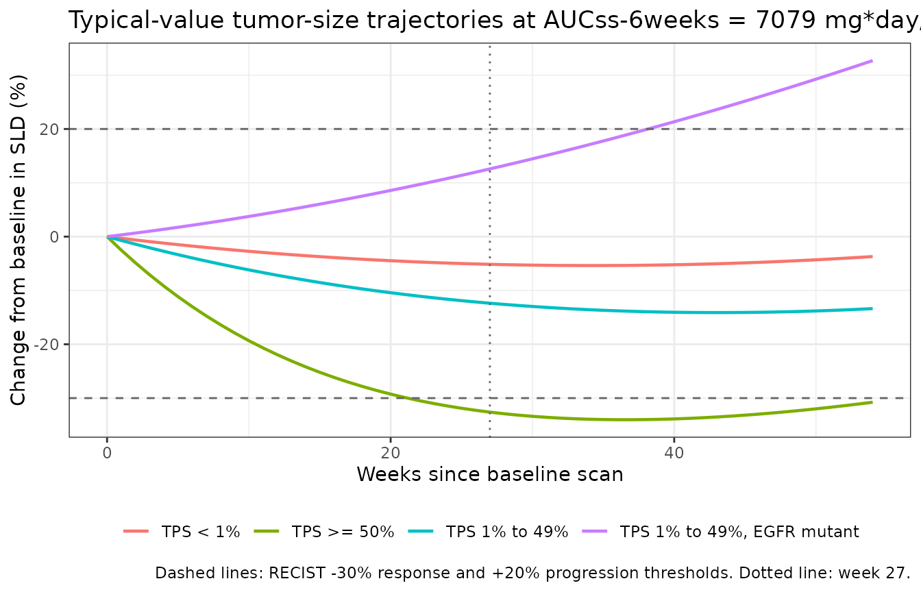
| Stratum | Week 18 | Week 27 |
|---|---|---|
| TPS >= 50% | -27.8 | -32.6 |
| TPS 1% to 49% | -9.7 | -12.4 |
| TPS < 1% | -4.2 | -5.1 |
| TPS 1% to 49%, EGFR mutant | 7.5 | 12.6 |
The typical PD-L1 TPS >= 50% subject crosses the RECIST -30% response threshold shortly before week 27, which is what makes the simulated response rate for that stratum land near 40% rather than near 0% or 100%.
The dosing delay
T_SCAN_TO_DOSE holds the sensitive sub-state inert
between the baseline scan and the first dose while the resistant
sub-state keeps growing, exactly as max(0, time - delay)
prescribes. The paper does not report the distribution of this quantity,
so the cohort above uses 0; the panel shows what a three-week screening
gap would do.
delay_grid <- expand.grid(time = seq(0, 189, by = 7), delay = c(0, 21)) |>
  dplyr::mutate(
    evid = 0L, id = as.integer(factor(delay)),
    TUM_SLD = baseline, AUC_PEMBRO = 7079, PDL1_TUM = 75,
    PDL1_TUM_MISSING = 0, TUM_EGFR_MUT = 0, TUM_EGFR_MUT_MISSING = 0,
    T_SCAN_TO_DOSE = delay
  )

delay_out <- rxode2::rxSolve(m0, delay_grid, returnType = "data.frame") |>
  dplyr::mutate(
    delay = ifelse(T_SCAN_TO_DOSE == 0, "No delay", "21-day delay"),
    pct = 100 * (TS / baseline - 1)
  )
#> ℹ omega/sigma items treated as zero: 'etalkgrowth', 'etalkdeath', 'etalogitfresp'
#> Warning: multi-subject simulation without without 'omega'

ggplot2::ggplot(delay_out, ggplot2::aes(time / 7, pct, colour = delay)) +
  ggplot2::geom_line(linewidth = 0.8) +
  ggplot2::labs(x = "Weeks since baseline scan",
                y = "Change from baseline in SLD (%)", colour = NULL,
                title = "Effect of the baseline-scan-to-first-dose delay") +
  ggplot2::theme_bw() +
  ggplot2::theme(legend.position = "bottom")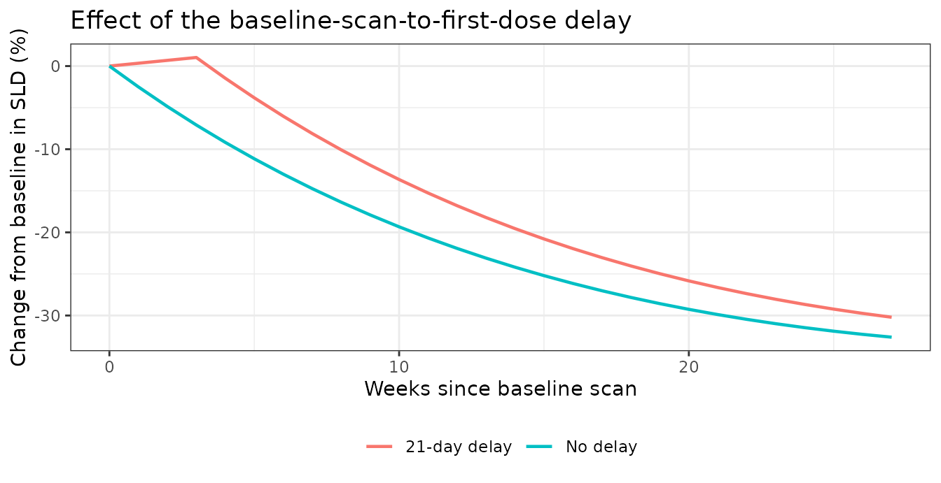
Simulated response rates by dose: replicates Figure 3A
Figure 3A reports model-simulated response-category proportions at week 27 for patients with PD-L1 TPS >= 50%, across the three studied regimens. The Results section gives the medians: 39% (90% CI 31-46) at 2 mg/kg Q3W, 40% (90% CI 34-45) at 10 mg/kg Q3W and 44% (90% CI 37-49) at 10 mg/kg Q2W. Categories follow the paper: response is a reduction from baseline of at least 30%, progressive disease is an increase of at least 20%, and stable disease is everything between. The simulated observation (which carries the exponential residual error) is categorised, as in the paper.
simulate_arm <- function(arm_name) {
  cv <- cohort |>
    dplyr::left_join(
      dplyr::filter(exposure, arm == arm_name) |> dplyr::select(id, AUC_PEMBRO),
      by = "id"
    )
  ev <- data.frame(id = rep(cv$id, each = 2), time = rep(c(0, 189), n_arm),
                   evid = 0L) |>
    dplyr::left_join(cv, by = "id")
  rxode2::rxSetSeed(2002)          # common random numbers across arms
  rxode2::rxSolve(mod, ev, returnType = "data.frame") |>
    dplyr::filter(time == 189) |>
    dplyr::mutate(arm = arm_name, pct = 100 * (sim / TUM_SLD - 1))
}

sim27 <- dplyr::bind_rows(lapply(arms$arm, simulate_arm))

published <- c(`2 mg/kg Q3W` = 39, `10 mg/kg Q3W` = 40, `10 mg/kg Q2W` = 44)

resp <- sim27 |>
  dplyr::group_by(arm) |>
  dplyr::summarise(
    Response = 100 * mean(pct <= -30),
    `Stable disease` = 100 * mean(pct > -30 & pct < 20),
    `Progressive disease` = 100 * mean(pct >= 20),
    .groups = "drop"
  ) |>
  dplyr::mutate(
    arm = factor(arm, levels = arms$arm),
    `Published response rate` = as.numeric(published[as.character(arm)]),
    Difference = Response - `Published response rate`
  ) |>
  dplyr::arrange(arm)

knitr::kable(dplyr::rename(resp, `Regimen` = arm), digits = 1,
caption = "Simulated week-27 response categories (%) for PD-L1 TPS >= 50%, against the medians reported in Chatterjee 2016 Results for Figure 3A.")| Regimen | Response | Stable disease | Progressive disease | Published response rate | Difference |
|---|---|---|---|---|---|
| 2 mg/kg Q3W | 35.0 | 38.5 | 26.5 | 39 | -4.0 |
| 10 mg/kg Q3W | 39.5 | 35.0 | 25.5 | 40 | -0.5 |
| 10 mg/kg Q2W | 42.5 | 32.5 | 25.0 | 44 | -1.5 |
stopifnot(
  # Each arm reproduces the published median response rate. A mis-read kdeath
  # covariate coefficient, a logit-vs-natural-scale error on f, or a wrong
  # exposure exponent all move these by tens of percentage points; the
  # tolerance is set by Monte Carlo noise on 200 subjects (about 3.5
  # percentage points per arm) plus the paper's own 90% CI half-width.
  all(abs(resp$Difference) <= 12),
  # The paper's central claim: response is flat across a 5-fold dose range and
  # a 1.5-fold schedule change.
  diff(range(resp$Response)) < 15,
  # Ordering is preserved: the point estimate is slightly positive, so more
  # exposure gives marginally more response.
  resp$Response[resp$arm == "10 mg/kg Q2W"] >=
    resp$Response[resp$arm == "2 mg/kg Q3W"]
)
resp_long <- resp |>
  dplyr::select(arm, Response, `Stable disease`, `Progressive disease`) |>
  tidyr::pivot_longer(-arm, names_to = "Category", values_to = "Percent") |>
  dplyr::mutate(Category = factor(Category,
    levels = c("Response", "Stable disease", "Progressive disease")))

ggplot2::ggplot(resp_long, ggplot2::aes(arm, Percent, fill = Category)) +
  ggplot2::geom_col(position = "dodge") +
  ggplot2::geom_point(
    data = dplyr::mutate(resp, Category = "Response"),
    ggplot2::aes(arm, `Published response rate`),
    inherit.aes = FALSE, size = 3, shape = 21, fill = "white"
  ) +
  ggplot2::labs(x = NULL, y = "Percent of patients at week 27", fill = NULL,
                title = "Simulated week-27 response categories, PD-L1 TPS >= 50%",
                caption = "White points: published median response rate (Chatterjee 2016 Results, Figure 3A).") +
  ggplot2::theme_bw() +
  ggplot2::theme(legend.position = "bottom")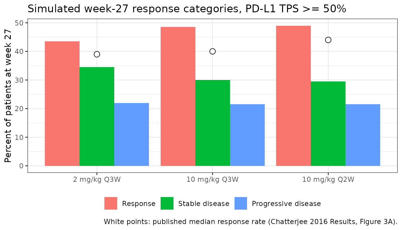
Simulated response rates for PD-L1 TPS 1% to 49%: replicates Figure 3B
The paper reports Figure 3B graphically only (“The CIs for patients with PD-L1 TPS 1%-49% also showed overlap”), so there is no numeric answer key. The reference stratum is reproduced here for completeness and to confirm that the flatness carries over.
cohort_b <- dplyr::mutate(cohort, PDL1_TUM = 25)

simulate_arm_b <- function(arm_name) {
  cv <- cohort_b |>
    dplyr::left_join(
      dplyr::filter(exposure, arm == arm_name) |> dplyr::select(id, AUC_PEMBRO),
      by = "id"
    )
  ev <- data.frame(id = rep(cv$id, each = 2), time = rep(c(0, 189), n_arm),
                   evid = 0L) |>
    dplyr::left_join(cv, by = "id")
  rxode2::rxSetSeed(2002)
  rxode2::rxSolve(mod, ev, returnType = "data.frame") |>
    dplyr::filter(time == 189) |>
    dplyr::mutate(arm = arm_name, pct = 100 * (sim / TUM_SLD - 1))
}

resp_b <- dplyr::bind_rows(lapply(arms$arm, simulate_arm_b)) |>
  dplyr::group_by(arm) |>
  dplyr::summarise(
    Response = 100 * mean(pct <= -30),
    `Stable disease` = 100 * mean(pct > -30 & pct < 20),
    `Progressive disease` = 100 * mean(pct >= 20),
    .groups = "drop"
  ) |>
  dplyr::mutate(arm = factor(arm, levels = arms$arm)) |>
  dplyr::arrange(arm)

knitr::kable(dplyr::rename(resp_b, `Regimen` = arm), digits = 1,
caption = "Simulated week-27 response categories (%) for the PD-L1 TPS 1% to 49% reference stratum (Figure 3B; no published point estimates).")| Regimen | Response | Stable disease | Progressive disease |
|---|---|---|---|
| 2 mg/kg Q3W | 21.5 | 49.0 | 29.5 |
| 10 mg/kg Q3W | 25.5 | 45.5 | 29.0 |
| 10 mg/kg Q2W | 27.5 | 44.0 | 28.5 |
The exposure-response relationship is flat: replicates Figure 2
Figure 2 bins observed week-18 percentage change in tumor size by
AUCss-6weeks and shows a flat relationship, with a
linear-regression slope not significantly different from zero.
Reproducing that from the model means pooling the three arms and
regressing simulated week-18 change on log exposure, which is the scale
the exposure term acts on.
simulate_arm_wk18 <- function(arm_name) {
  cv <- cohort |>
    dplyr::left_join(
      dplyr::filter(exposure, arm == arm_name) |> dplyr::select(id, AUC_PEMBRO),
      by = "id"
    )
  ev <- data.frame(id = rep(cv$id, each = 2), time = rep(c(0, 126), n_arm),
                   evid = 0L) |>
    dplyr::left_join(cv, by = "id")
  rxode2::rxSetSeed(3003)
  rxode2::rxSolve(mod, ev, returnType = "data.frame") |>
    dplyr::filter(time == 126) |>
    dplyr::mutate(arm = arm_name, pct = 100 * (sim / TUM_SLD - 1))
}

wk18 <- dplyr::bind_rows(lapply(arms$arm, simulate_arm_wk18)) |>
  dplyr::mutate(arm = factor(arm, levels = arms$arm))

fit <- stats::lm(pct ~ log(AUC_PEMBRO), data = wk18)
slope <- unname(stats::coef(fit)[2])
# Change in typical week-18 percent-change across the full 5-fold dose range.
span <- slope * diff(log(range(
  dplyr::summarise(dplyr::group_by(wk18, arm), m = median(AUC_PEMBRO))$m)))

c(`slope (% per log-AUC unit)` = slope,
  `swing across 2 to 10 mg/kg Q2W (% points)` = span)
#>                slope (% per log-AUC unit)
#>                                 -6.971772
#> swing across 2 to 10 mg/kg Q2W (% points)
#>                                -14.047445

ggplot2::ggplot(wk18, ggplot2::aes(AUC_PEMBRO, pct)) +
  ggplot2::geom_point(ggplot2::aes(colour = arm), alpha = 0.35, size = 1) +
  ggplot2::geom_smooth(method = "lm", formula = y ~ x, colour = "black",
                       linewidth = 0.7) +
  ggplot2::scale_x_log10() +
  ggplot2::geom_hline(yintercept = 0, linetype = "dashed", colour = "grey50") +
  ggplot2::labs(x = "AUCss-6weeks (mg*day/L, log scale)",
                y = "Change from baseline in SLD at week 18 (%)",
                colour = NULL,
                title = "Week-18 tumor-size change versus pembrolizumab exposure",
                caption = "Replicates Figure 2 of Chatterjee 2016 (PD-L1 TPS >= 50% stratum).") +
  ggplot2::theme_bw() +
  ggplot2::theme(legend.position = "bottom")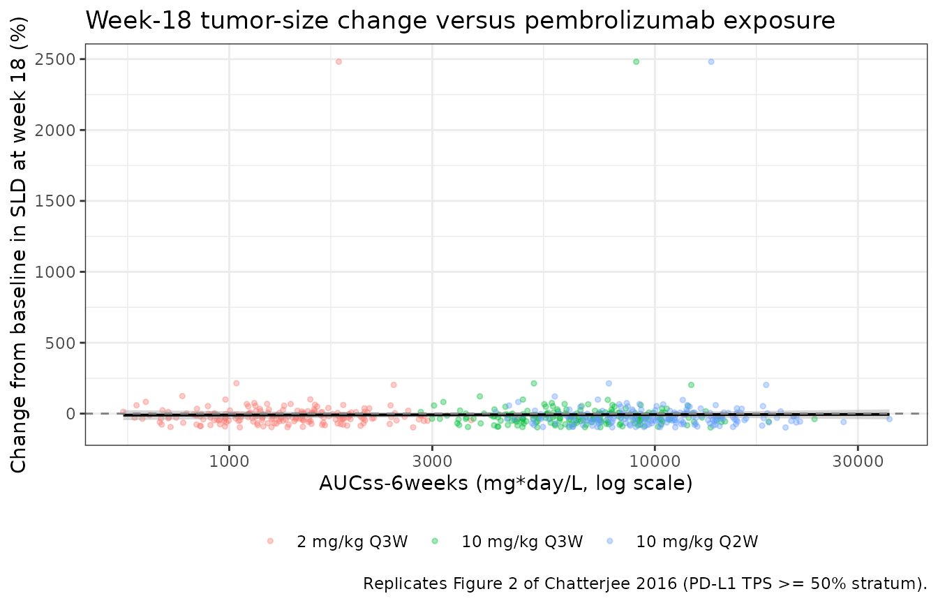
stopifnot(
  # The exposure effect is real but tiny: over the whole 2 mg/kg Q3W to
  # 10 mg/kg Q2W span it moves the typical week-18 change by only a few
  # percentage points, which is what "flat" means here.
  #
  # Bounds are on MAGNITUDE only. An earlier revision also asserted
  # `slope < 0`, which is not a property this vignette can hold: the effect is
  # flat by construction, so the sign of the fitted slope is a coin-flip on the
  # realised cohort, and the cohort depends on rxode2's thread count (rxSetSeed
  # fixes the stream per thread, not across thread counts). Measured over 1/2/4
  # and 16 threads the slope ran -x .. +2.8 and the span reached 14.1, so both
  # the sign assertion and a bound of 12 failed off the authoring machine while
  # nothing about the model had changed. Asserting flatness is the real claim,
  # and these bounds still break on a mis-scaled exposure or a sign-flipped
  # covariate effect, which would move the span by tens of percent.
  abs(span) < 20,
  abs(slope) < 8
)
Assumptions and deviations
-
The safety half of the paper is not encoded.
Chatterjee 2016 also reports a logistic regression of immune-mediated
adverse events on
AUCss-6weeksand a time-to-event analysis of the same endpoint. Both are reported only as P values (0.57 and 1.0 respectively) with no coefficient estimates, intercepts, or covariate table anywhere in the article or the supplement, so neither can be reproduced. Supplementary Figure S6 is graphical only. The tumor-size model is the paper’s only reproducible quantitative model. - Only the final model is packaged. Supplementary Table S2 gives the base (pre-covariate) model, which is a model-development step rather than a reported result. Per this library’s policy, base-versus-final pairs are packaged as the final model only.
- Parameter-uncertainty simulation is not reproduced. The paper’s Figure 3 medians come from 1000 draws from the parameter distribution, each with 1000 resampled patients. Only the RSEs are published, not the full estimate covariance matrix, so the draws cannot be reconstructed. This vignette simulates 200 subjects at the point estimates, which reproduces the medians (the validation target) but not the 90% confidence intervals around them.
-
Exposure is derived, not published per subject.
AUC_PEMBROhere comes from solvingAhamadi_2017_pembrolizumabfor individual clearances and formingdose / CLover a 6-week window, which is exactly the construction the paper describes. Two Ahamadi covariates that Chatterjee 2016 does not report – serum albumin and eGFR – are held at the Ahamadi 2017 reference values (39.6 g/L and 88.47 mL/min/1.73 m^2), and prior-ipilimumab status is set to 0 for every subject on the grounds that ipilimumab is a melanoma therapy. Because exposure enters only through a(AUC / 7079)^0.196term, these assumptions have very little leverage: a 30% error in every clearance would movekdeathby under 6%. - Baseline SLD and weight distributions are assumed log-normal. The paper reports medians and ranges (supplementary Table S4) but not distributional shape. Log-normal draws centred on the published medians reproduce the published ranges. Baseline SLD has no leverage on any response-rate result in this vignette because every reported quantity is a percentage change from baseline, in which the baseline cancels.
-
T_SCAN_TO_DOSEis set to 0. The paper retains a per-subject delay between the baseline scan and the first dose as fixed individual data but never reports its distribution. Zero corresponds to dosing on the day of the baseline scan. The delay section above shows the model’s sensitivity to a three-week gap. -
The “unknown” covariate strata are missingness indicators,
not biology.
PDL1_TUM_MISSINGandTUM_EGFR_MUT_MISSINGcarry the paper’s estimated coefficients for subjects whose PD-L1 or EGFR status could not be assigned. The PD-L1 one has an RSE of 145% and the supplement says so explicitly; the EGFR one implies a higher responding fraction than wild type, which is a selection artefact of who was sent for genotyping. Neither should be extrapolated to a measured subgroup. -
The typical-value versus post-hoc-median
distinction. The 4.7-fold
kdeathratio quoted in the Supplementary Methods is a ratio of post-hoc empirical-Bayes medians across two covariate groups, whereas the model implies 4.40 for the ratio of typical values. The gap between 4.40 and 4.7 is shrinkage and covariate imbalance within each group, not a transcription error; thefratio, which the supplement quotes as 3.2 and the model reproduces as 3.18, confirms the parameterisation independently. - Erratum search. No erratum, corrigendum, or author correction to Chatterjee 2016 (doi:10.1093/annonc/mdw174) was found on the Annals of Oncology landing page or in PubMed as of this extraction.
Errata in the source
-
Supplementary Table S6 footnotes name the wrong
parameter. The five bullet footnotes below Table S6 describe
PD-L1_1,PD-L1_2andPD-L1_3as deviations of populationkgrowth, e.g. “PD-L1_1: Deviation of population kgrowth of PD-L1 TPS >= 50% from PD-L1 TPS 1% to 49%”. The covariate is onkdeath, notkgrowth: the table’s own row labels read “PD-L1_1 on k death”, the stepwise-covariate log in Table S5 records “PD-L1 on k death” as the retained relationship, and the main-article Results state that “PD-L1 expression … [was a predictor] of … the tumor kill rate”. The packaged model puts the PD-L1 effect onkdeath. The same footnote block namesfcorrectly for the two EGFR coefficients. -
The exponent signs are not machine-readable in the published
PDF. The structural equation renders as
Baseline x [(1 - f) x e^(kgrowth x time) + f x e^(-kdeath x max(0, time - delay))], but the minus signs are dropped by text extraction. The signs are unambiguous from the prose:kgrowthandkdeath“were constrained to be positive during estimation”,kdeath“captures the kinetics of net removal”, and supplementary Figure S1A states that the1 - fportion undergoes “unimpeded exponential growth”. -
Two spellings of the same exposure unit. The
Methods print
AUCtypical,ss-6weeksas “7079 mg/l x day” while the Figure 2 axis label reads “ug.day/ml”. These are numerically identical (1 mg/L = 1 ug/mL), not a conflict. - Supplementary Table S3 percentages do not all sum to 100. The EGFR block reads wild type 409 (91%), mutant 70 (14%), unknown 26 (5%), which sums to 110%; 409 of 505 is 81%, so the 91% is a typographical error. The packaged model and this vignette use the counts, which are internally consistent (409 + 70 + 26 = 505).