Cyclophosphamide / phosphoramide mustard (Jaber 2023)
Source:vignettes/articles/Jaber_2023_cyclophosphamide.Rmd
Jaber_2023_cyclophosphamide.RmdModel and source
- Citation: Jaber MM, Takahashi T, Kirstein MN, Al-Kofahi M, Jacobson PA, Brundage RC. Influence of Renal Function on Phosphoramide Mustard Exposure: A Nonlinear Mixed-Effects Analysis. J Clin Pharmacol. 2023;63(1):135-141. doi:10.1002/jcph.2144
- Description: Population PK model for phosphoramide mustard, the cytotoxic end metabolite of cyclophosphamide, after a single 2-h intravenous infusion of cyclophosphamide 50 mg/kg in adults undergoing allogeneic hematopoietic cell transplantation (Jaber 2023). Formation is delayed through two transit compartments sharing one rate constant (cyclophosphamide, then 4-hydroxycyclophosphamide) into a one-compartment phosphoramide mustard disposition with parallel linear renal clearance, proportional to weight-normalised Cockcroft-Gault creatinine clearance, and Michaelis-Menten metabolic elimination; theory-based allometry on total body weight. Only phosphoramide mustard was measured, so its clearance and volume are apparent (scaled by the fraction of the cyclophosphamide dose converted).
- Article: https://doi.org/10.1002/jcph.2144 (open access, PMC10087276)
The supporting information holds the final NONMEM control stream
(whose $THETA and $OMEGA blocks carry the
final estimates of Table 2 to more digits), the Julia simulation script
behind Table 3 and Figures S2-S4, and Figures S1-S4. A literature check
on 2026-10-26 (Europe PMC) found no erratum or correction for this
article.
Only phosphoramide mustard (PM) was measured. Cyclophosphamide and 4-hydroxycyclophosphamide enter the model as two amount-only transit compartments that share one rate constant and serve only to delay the appearance of PM; the authors caution that this rate constant should not be interpreted mechanistically. Because the fraction of the cyclophosphamide dose converted to PM is not identifiable, the PM clearance, volume and Vmax are apparent values scaled by that fraction.
Population
Jaber 2023 analysed 85 of 110 adults enrolled in a single-centre observational PK study at the University of Minnesota. All had a high-risk hematologic malignancy (leukemia 49%, myelodysplastic syndrome 19%, lymphoma 11%, other 21%) and received a reduced-intensity conditioning regimen for allogeneic hematopoietic cell transplantation: a single dose of cyclophosphamide 50 mg/kg infused over 2 h on day -7, fludarabine on days -6 to -2 and 200 cGy total body irradiation on day -1. The dose was based on total body weight, or on adjusted body weight for patients whose weight exceeded 150% of ideal body weight (28%). Median age was 63 years (21-75), median weight 84 kg (47-177), 45% were female and median Cockcroft-Gault creatinine clearance was 77 mL/min (32-150) (Table 1). PM was sampled at 0, 4, 6, 8, 23, 26 and 47 h after the start of the infusion; 506 concentrations were analysed, 11.4% of them below the 50 ng/mL limit of quantification.
The same information is available programmatically via
readModelDb("Jaber_2023_cyclophosphamide")()$population.
Source trace
The per-parameter origin is recorded as an in-file comment next to
each ini() entry in
inst/modeldb/specificDrugs/Jaber_2023_cyclophosphamide.R.
| Equation / parameter | Value | Source location |
|---|---|---|
lcl_renal (renal clearance, 70 kg, CrCL 85 mL/min) |
log(14.9) L/h | Table 2; NONMEM $THETA(1) 14.913 |
lvc (apparent volume, 70 kg) |
log(525) L | Table 2; $THETA(2) 524.657 |
lktr (shared transit rate constant, 70 kg) |
log(1.3) 1/h | Table 2; $THETA(3) 1.30505 |
lvmax (Michaelis-Menten Vmax, 70 kg) |
log(81.2) mg/h | Table 2; $THETA(7) 81.2164 |
lkm (Michaelis-Menten Km) |
log(0.51) mg/L | Table 2; $THETA(8) 0.514354 |
e_crcl_cl_renal |
1 (held constant) | Methods after Equation 3 (estimated 0.97, then set to 1); Table 2;
$THETA(4) 1 FIX
|
e_wt_cl_renal, e_wt_vmax
|
0.75 (held constant) | Equations 3-4; Table 2 |
e_wt_vc |
1 (held constant) | Methods “Theory-based allometry”; Table 2 |
e_wt_ktr |
0.25 (held constant) | Equation 2; Table 2 |
etalcl_renal, etalvc,
etalktr, etalkm
|
0.15861, 0.108285, 0.0744403, 0.0842706 | NONMEM $OMEGA; Table 2 BSV 39.8, 32.9, 27.3, 29.0% (=
100 x sqrt(omega^2)) |
propSd, addSd
|
0.097, 54.9 ng/mL | Table 2; $THETA(5), $THETA(6);
$ERROR SD = sqrt(PROP^2 + ADD^2) |
| Cockcroft-Gault CrCL, female factor 0.85, cap at 150 mL/min | n/a | Methods “Model Development”; NONMEM $PK
|
Renal clearance
cl_renal = CL * ((CrCL/85) * (70/WT))^1 * (WT/70)^0.75
|
n/a | Equation 3; NONMEM $PK
|
Metabolic elimination vmax * C / (km + C)
|
n/a | Equations 4-6; NONMEM $DES
|
d/dt(depot_iv), d/dt(transit1),
d/dt(central)
|
n/a | Equations 7-9; NONMEM $DES (A(1), A(3), A(2)) |
Cc = central / vc * 1000 (ng/mL) |
n/a | NONMEM $PK S2 = V/1000
|
Virtual cohort
The original data are not public. The cohort below approximates Table 1. Age, weight and serum creatinine are drawn so the derived Cockcroft-Gault creatinine clearance spans roughly the observed range; height is drawn only to decide which patients are dosed on adjusted body weight.
set.seed(20230101)
n_sub <- 200

cohort <- tibble(
  id = seq_len(n_sub),
  SEXF = rbinom(n_sub, 1, 0.45),
  AGE = pmin(pmax(round(rnorm(n_sub, 60, 11)), 21), 75),
  WT = pmin(pmax(exp(rnorm(n_sub, log(84), 0.22)), 47), 177),
  CREAT = pmin(pmax(exp(rnorm(n_sub, log(1.1), 0.25)), 0.4), 2.0),
  HT_cm = ifelse(SEXF == 1, rnorm(n_sub, 163, 7), rnorm(n_sub, 177, 7))
) |>
  mutate(
    # Devine ideal body weight; adjusted body weight when WT > 150% of IBW
    # (Jaber 2023 Equation 1).
    IBW = ifelse(SEXF == 1, 45.5, 50) + 2.3 * (HT_cm / 2.54 - 60),
    adjusted = WT > 1.5 * IBW,
    dose_wt = ifelse(adjusted, IBW + 0.5 * (WT - IBW), WT),
    amt = 50 * dose_wt,
    crcl = pmin((140 - AGE) * WT / (72 * CREAT) * 0.85^SEXF, 150)
  )

cohort |>
  summarise(
    `Age median (range)` = sprintf("%.0f (%.0f-%.0f)", median(AGE), min(AGE), max(AGE)),
    `Weight median (range), kg` = sprintf("%.0f (%.0f-%.0f)", median(WT), min(WT), max(WT)),
    `Female, %` = sprintf("%.0f", 100 * mean(SEXF)),
    `CrCL median (range), mL/min` = sprintf("%.0f (%.0f-%.0f)", median(crcl), min(crcl), max(crcl)),
    `Dosed on adjusted weight, %` = sprintf("%.0f", 100 * mean(adjusted))
  ) |>
  tidyr::pivot_longer(everything(), names_to = "Characteristic", values_to = "Virtual cohort") |>
  mutate(`Jaber 2023 Table 1` = c("63 (21-75)", "84 (47-177)", "45", "77 (32-150)", "28")) |>
knitr::kable(caption = "Virtual cohort against Table 1.")| Characteristic | Virtual cohort | Jaber 2023 Table 1 |
|---|---|---|
| Age median (range) | 61 (23-75) | 63 (21-75) |
| Weight median (range), kg | 83 (51-149) | 84 (47-177) |
| Female, % | 48 | 45 |
| CrCL median (range), mL/min | 77 (34-150) | 77 (32-150) |
| Dosed on adjusted weight, % | 34 | 28 |
Every patient receives one 2-h infusion of cyclophosphamide 50 mg/kg
into depot_iv. Observations are on the PM state
central; the model returns the PM concentration
Cc (ng/mL) at those rows.
obs_times <- sort(unique(c(seq(0, 100, by = 0.5), 4, 6, 8, 23, 26, 47)))

dose_rows <- cohort |>
  transmute(id, time = 0, amt, dur = 2, evid = 1L, cmt = "depot_iv",
            SEXF, AGE, WT, CREAT)
obs_rows <- cohort |>
  select(id, SEXF, AGE, WT, CREAT) |>
  tidyr::crossing(time = obs_times) |>
  mutate(amt = 0, dur = 0, evid = 0L, cmt = "central")
events <- bind_rows(dose_rows, obs_rows) |>
  arrange(id, time, desc(evid)) |>
  mutate(treatment = "CY 50 mg/kg")
stopifnot(!anyDuplicated(events[events$evid == 0, c("id", "time")]))
Simulation
mod <- readModelDb("Jaber_2023_cyclophosphamide")
sim <- rxode2::rxSolve(mod, events = events, keep = c("treatment", "WT")) |>
  as.data.frame()
#> ℹ parameter labels from comments will be replaced by 'label()'
Replicate published figures
Figure S1: observed PM concentrations
Figure S1 of Jaber 2023 plots the 506 observed PM concentrations. The simulated 5th, 50th and 95th percentiles of the virtual cohort (with residual error) at the protocol sampling times should cover that cloud: most early (4-8 h) observations lie between about 2,500 and 9,000 ng/mL and most 23-26 h observations between the 50 ng/mL limit of quantification and about 2,500 ng/mL.
set.seed(20230102)
sim_vpc <- rxode2::rxSolve(
  mod,
  events = events |> filter(evid == 1 | time %in% c(4, 6, 8, 23, 26, 47)),
  keep = c("treatment")
) |>
  as.data.frame()

vpc <- sim_vpc |>
  group_by(time) |>
  summarise(
    Q05 = quantile(sim, 0.05), Q50 = quantile(sim, 0.50), Q95 = quantile(sim, 0.95),
    .groups = "drop"
  )
knitr::kable(vpc, digits = 0,
caption = "Simulated PM concentration percentiles (ng/mL) at the sampling times.")| time | Q05 | Q50 | Q95 |
|---|---|---|---|
| 4 | 2728 | 4740 | 8392 |
| 6 | 2979 | 4841 | 8344 |
| 8 | 2578 | 4353 | 8075 |
| 23 | 666 | 1684 | 2797 |
| 26 | 359 | 1255 | 2195 |
| 47 | -80 | 32 | 284 |
ggplot(vpc, aes(time, Q50)) +
  geom_ribbon(aes(ymin = pmax(Q05, 1), ymax = Q95), alpha = 0.25) +
  geom_line() +
  geom_point() +
  geom_hline(yintercept = 50, colour = "red", linetype = "dashed") +
  labs(x = "Time after start of infusion (h)", y = "PM concentration (ng/mL)",
       title = "Simulated 5th-50th-95th percentiles with residual error",
       caption = "Compare with Figure S1 of Jaber 2023; red line is the 50 ng/mL LLOQ.")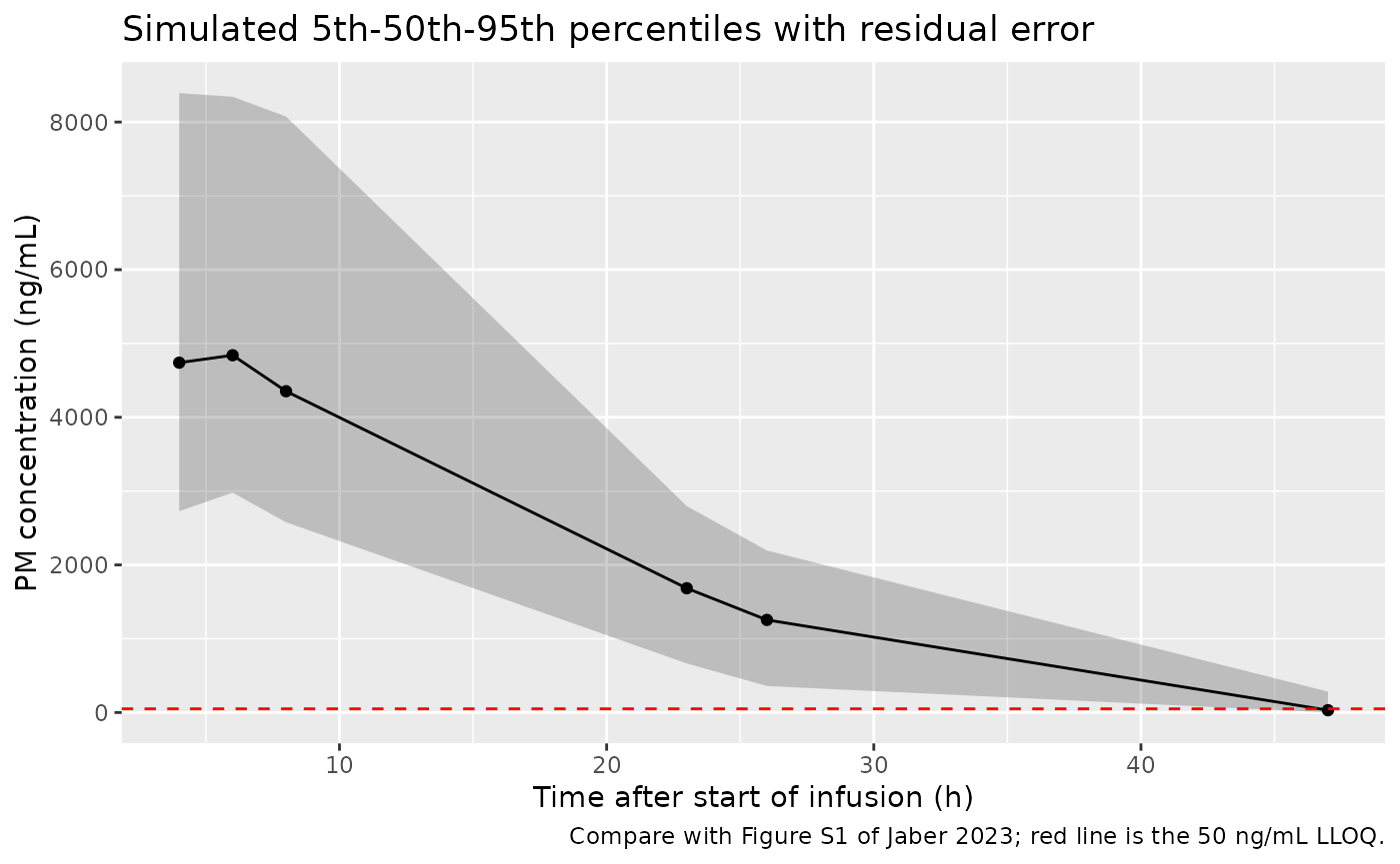
# The early median sits in the middle of the Figure S1 cloud and the 23 h
# median well below the early peak; a mis-scaled volume or dose moves both by
# tens of percent.
early_med <- vpc$Q50[vpc$time == 6]
late_med <- vpc$Q50[vpc$time == 23]
stopifnot(early_med > 3000, early_med < 7500, late_med > 300, late_med < 2500)
Figure S3 and Table 3: effect of creatinine clearance on PM exposure
The paper’s sensitivity analysis uses a 70-kg typical patient who receives 3,500 mg of cyclophosphamide (50 mg/kg), with creatinine clearance set directly to 30-120 mL/min. In the supplementary Julia script the whole dose is placed in the cyclophosphamide compartment at time zero, rather than infused over 2 h, so the replication does the same. In this model creatinine clearance is computed from serum creatinine, so the serum creatinine that gives each target clearance is back-calculated for a 63-year-old man.
mod_typical <- rxode2::zeroRe(mod)
#> ℹ parameter labels from comments will be replaced by 'label()'
target_crcl <- seq(30, 120, by = 10)

typical_events <- function(crcl_target, end = 100) {
  rxode2::et(amt = 3500, cmt = "depot_iv") |>
    rxode2::et(seq(0, end, by = 0.05), cmt = "central") |>
    as.data.frame() |>
    mutate(id = crcl_target, WT = 70, AGE = 63, SEXF = 0,
           CREAT = (140 - 63) * 70 / (72 * crcl_target))
}
typ_ev <- bind_rows(lapply(target_crcl, typical_events))

trap <- function(t, y) sum(diff(t) * (head(y, -1) + tail(y, -1)) / 2)

solve_typical <- function(vmax_mg_h) {
  rxode2::rxSolve(mod_typical, events = typ_ev,
                  params = c(lvmax = log(vmax_mg_h))) |>
    as.data.frame() |>
    rename(crcl_target = id) |>
    mutate(crcl_target = as.numeric(as.character(crcl_target)))
}
sim_typ <- solve_typical(81.2)
#> ℹ omega/sigma items treated as zero: 'etalcl_renal', 'etalvc', 'etalktr', 'etalkm'
#> Warning: multi-subject simulation without without 'omega'
fig_s3 <- sim_typ |>
  filter(crcl_target %in% c(30, 60, 120), time <= 48) |>
  group_by(crcl_target) |>
  arrange(time, .by_group = TRUE) |>
  mutate(auc = c(0, cumsum(diff(time) * (head(Cc, -1) + tail(Cc, -1)) / 2))) |>
  ungroup()

ggplot(fig_s3, aes(time, auc, colour = factor(crcl_target))) +
  geom_line() +
  scale_x_continuous(breaks = seq(0, 48, 8)) +
  labs(x = "Time (h)", y = "PM AUC (ng*h/mL)", colour = "CrCL (mL/min)",
       caption = "Replicates Figure S3 of Jaber 2023.")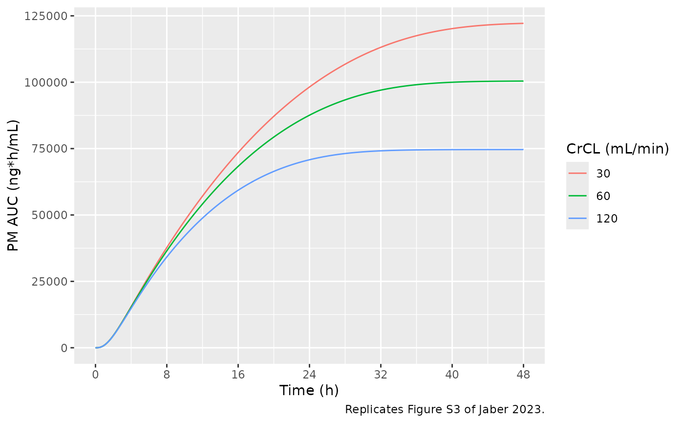
auc48 <- fig_s3 |>
  group_by(crcl_target) |>
  summarise(auc48 = max(auc), .groups = "drop") |>
  # Plateau values read by the maintainers from Figure S3.
  mutate(figure_s3 = c(`30` = 122000, `60` = 100500, `120` = 75000)[as.character(crcl_target)],
         pct_diff = 100 * (auc48 / figure_s3 - 1))
knitr::kable(auc48, digits = c(0, 0, 0, 1),
caption = "AUC0-48 h of the typical 70-kg patient against Figure S3.")| crcl_target | auc48 | figure_s3 | pct_diff |
|---|---|---|---|
| 30 | 122161 | 122000 | 0.1 |
| 60 | 100427 | 100500 | -0.1 |
| 120 | 74641 | 75000 | -0.5 |
# Deterministic typical-value solve against a figure read to about 1%.
stopifnot(all(abs(auc48$pct_diff) < 4))
Table 3 reports the percentage increase in AUC0-8 h and in AUC0-100 h (approximately AUC to infinity) relative to a creatinine clearance of 120 mL/min. The table below compares Table 3 with the model as published (Vmax 81.2 mg/h) and with the same model at Vmax 40.2 mg/h, the value written into the supplementary Julia function that generated Table 3.
pct_increase <- function(sims) {
  sims |>
    group_by(crcl_target) |>
    summarise(auc8 = trap(time[time <= 8], Cc[time <= 8]),
              auc100 = trap(time, Cc), .groups = "drop") |>
    mutate(inc8 = 100 * (auc8 / auc8[crcl_target == 120] - 1),
           inc100 = 100 * (auc100 / auc100[crcl_target == 120] - 1))
}
published_t3 <- tibble(
  crcl_target = target_crcl,
  t3_inc8 = c(10.4, 9.2, 8.0, 6.8, 5.6, 4.4, 3.3, 2.1, 1.1, 0),
  t3_inc100 = c(102.3, 80.9, 63.9, 49.9, 38.2, 28.3, 19.7, 12.3, 5.8, 0)
)
t3 <- pct_increase(sim_typ) |>
  select(crcl_target, inc8, inc100) |>
  left_join(pct_increase(solve_typical(40.2)) |>
              select(crcl_target, inc8_v40 = inc8, inc100_v40 = inc100),
            by = "crcl_target") |>
  left_join(published_t3, by = "crcl_target")
#> ℹ omega/sigma items treated as zero: 'etalcl_renal', 'etalvc', 'etalktr', 'etalkm'
#> Warning: multi-subject simulation without without 'omega'

t3 |>
  select(crcl_target, t3_inc8, inc8, t3_inc100, inc100, inc100_v40) |>
  rename(
    "CrCL (mL/min)" = crcl_target,
    "Table 3 AUC0-8 increase (%)" = t3_inc8,
    "Model AUC0-8 increase (%)" = inc8,
    "Table 3 AUC increase (%)" = t3_inc100,
    "Model AUC increase (%), Vmax 81.2" = inc100,
    "AUC increase (%), Vmax 40.2" = inc100_v40
  ) |>
knitr::kable(digits = 1, caption = "Table 3 of Jaber 2023 against the packaged model.")| CrCL (mL/min) | Table 3 AUC0-8 increase (%) | Model AUC0-8 increase (%) | Table 3 AUC increase (%) | Model AUC increase (%), Vmax 81.2 | AUC increase (%), Vmax 40.2 |
|---|---|---|---|---|---|
| 30 | 10.4 | 10.4 | 102.3 | 64.1 | 102.3 |
| 40 | 9.2 | 9.2 | 80.9 | 52.8 | 80.9 |
| 50 | 8.0 | 7.9 | 63.9 | 43.1 | 63.8 |
| 60 | 6.8 | 6.8 | 49.9 | 34.6 | 49.9 |
| 70 | 5.6 | 5.6 | 38.2 | 27.1 | 38.2 |
| 80 | 4.4 | 4.4 | 28.3 | 20.5 | 28.3 |
| 90 | 3.3 | 3.3 | 19.7 | 14.6 | 19.7 |
| 100 | 2.1 | 2.2 | 12.3 | 9.2 | 12.3 |
| 110 | 1.1 | 1.1 | 5.8 | 4.4 | 5.8 |
| 120 | 0.0 | 0.0 | 0.0 | 0.0 | 0.0 |
# AUC0-8 h hardly depends on Vmax, and the model reproduces the Table 3
# column to rounding. The total-AUC column is reproduced to rounding only at
# Vmax 40.2 mg/h; that it is NOT reproduced at the published Vmax is the
# documented deviation below, so the published-Vmax total AUC is not gated.
stopifnot(
  all(abs(t3$inc8 - t3$t3_inc8) < 0.25),
  all(abs(t3$inc100_v40 - t3$t3_inc100) < 0.25)
)
Figures S2 and S4: elimination routes
The renal (linear) and metabolic (Michaelis-Menten) elimination rates are integrated over 0-100 h for the same typical patient.
routes <- sim_typ |>
  group_by(crcl_target) |>
  summarise(
    renal = trap(time, kel * central),
    metabolic = trap(time, vmax * cpm_mgl / (km + cpm_mgl)),
    .groups = "drop"
  ) |>
  mutate(pct_renal = 100 * renal / 3500, pct_metabolic = 100 * metabolic / 3500)

# Percent renal at the five plotted CrCL values, read by the maintainers from
# Figure S4.
fig_s4 <- tibble(crcl_target = c(30, 50, 80, 100, 120),
                 figure_s4_renal = c(18.5, 27, 36, 41, 45))
s4 <- inner_join(routes, fig_s4, by = "crcl_target")
s4 |>
  select(crcl_target, figure_s4_renal, pct_renal, pct_metabolic) |>
  rename("CrCL (mL/min)" = crcl_target,
         "Figure S4 renal (%)" = figure_s4_renal,
         "Model renal (%)" = pct_renal,
         "Model metabolic (%)" = pct_metabolic) |>
knitr::kable(digits = 1, caption = "Share of the dose eliminated by each route against Figure S4.")| CrCL (mL/min) | Figure S4 renal (%) | Model renal (%) | Model metabolic (%) |
|---|---|---|---|
| 30 | 18.5 | 18.4 | 81.6 |
| 50 | 27.0 | 26.7 | 73.3 |
| 80 | 36.0 | 36.0 | 64.0 |
| 100 | 41.0 | 40.8 | 59.2 |
| 120 | 45.0 | 44.9 | 55.1 |
stopifnot(all(abs(s4$pct_renal - s4$figure_s4_renal) < 2))

routes |>
  select(crcl_target, Renal = pct_renal, `Non-renal` = pct_metabolic) |>
  tidyr::pivot_longer(-crcl_target, names_to = "route", values_to = "pct") |>
  ggplot(aes(crcl_target, pct, colour = route)) +
  geom_line() + geom_point() +
  coord_cartesian(ylim = c(0, 100)) +
  labs(x = "CrCL (mL/min)", y = "Dose eliminated (%)", colour = NULL,
       caption = "Replicates Figure S4 of Jaber 2023.")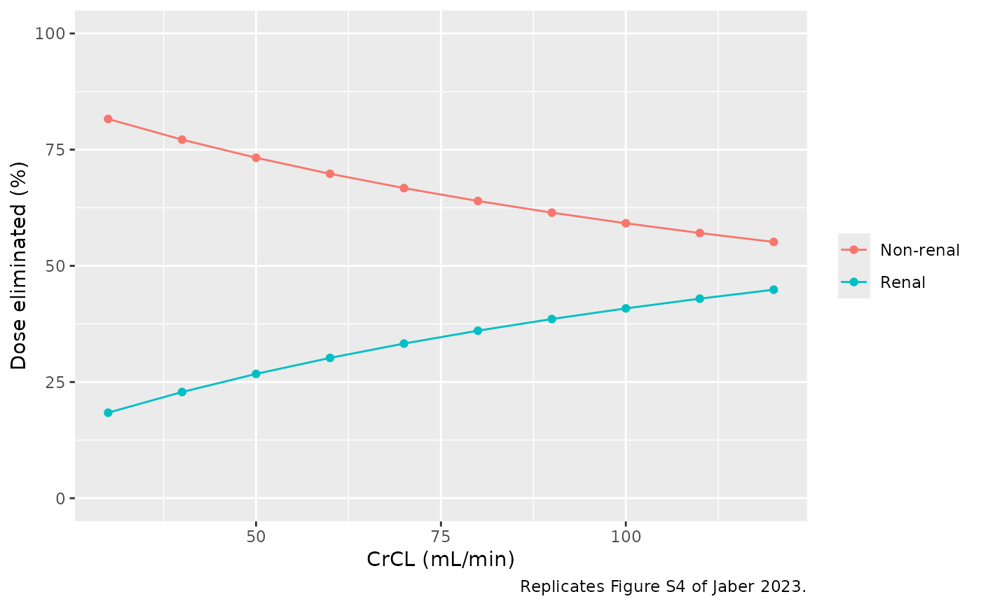
sim_typ |>
  filter(crcl_target %in% c(30, 60, 120)) |>
  group_by(crcl_target) |>
  arrange(time, .by_group = TRUE) |>
  mutate(eliminated = c(0, cumsum(diff(time) * (
    head(kel * central + vmax * cpm_mgl / (km + cpm_mgl), -1) +
      tail(kel * central + vmax * cpm_mgl / (km + cpm_mgl), -1)) / 2))) |>
  ungroup() |>
  ggplot(aes(time, eliminated, colour = factor(crcl_target))) +
  geom_line() +
  geom_hline(yintercept = 3500, linetype = "dashed") +
  labs(x = "Time (h)", y = "Cumulative amount eliminated (mg)", colour = "CrCL (mL/min)",
       caption = "Replicates Figure S2 of Jaber 2023.")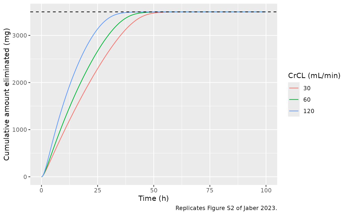
PKNCA validation
NCA on the dense simulated profiles of the virtual cohort (with between-subject variability, without residual error). The paper reports no NCA table. Its Discussion places the PM AUC0-8 h threshold for higher nonrelapse mortality, 34,235 ngh/mL from the authors’ earlier analysis of this cohort, at about 20% above the median, which implies a cohort median AUC0-8 h of roughly 28,500 ngh/mL; that derived value is the only reference available.
sim_nca <- sim |>
  filter(!is.na(Cc)) |>
  select(id, time, Cc, treatment)
stopifnot(all(tapply(sim_nca$time, sim_nca$id, min) == 0))

conc_obj <- PKNCA::PKNCAconc(sim_nca, Cc ~ time | treatment + id)
dose_df <- events |>
  filter(evid == 1) |>
  select(id, time, amt, dur, treatment)
dose_obj <- PKNCA::PKNCAdose(dose_df, amt ~ time | treatment + id, duration = "dur")

intervals <- data.frame(
  start = c(0, 0),
  end = c(8, Inf),
  auclast = c(TRUE, FALSE),
  cmax = c(FALSE, TRUE),
  tmax = c(FALSE, TRUE),
  aucinf.obs = c(FALSE, TRUE),
  half.life = c(FALSE, TRUE)
)
nca_res <- PKNCA::pk.nca(PKNCA::PKNCAdata(conc_obj, dose_obj, intervals = intervals))
summary(nca_res)
#>  start end   treatment   N      auclast        cmax              tmax
#>      0   8 CY 50 mg/kg 200 28700 [33.8]           .                 .
#>      0 Inf CY 50 mg/kg 200            . 5130 [33.5] 5.00 [3.50, 8.00]
#>    half.life   aucinf.obs
#>            .            .
#>  2.45 [1.12] 87000 [30.0]
#>
#> Caption: auclast, cmax, aucinf.obs: geometric mean and geometric coefficient of variation; tmax: median and range; half.life: arithmetic mean and standard deviation; N: number of subjects
published <- tibble::tibble(treatment = "CY 50 mg/kg", auclast = 34235 / 1.2)
cmp <- nlmixr2lib::ncaComparisonTable(
  simulated = nca_res,
  reference = published,
  by = "treatment",
  units = c(auclast = "ng*h/mL"),
  tolerance_pct = 20
)
knitr::kable(cmp, caption = "Simulated median AUC0-8 h against the value implied by the Discussion. * differs by >20%.")| NCA parameter | treatment | Reference | Simulated | % diff |
|---|---|---|---|---|
| AUClast (ng*h/mL) | CY 50 mg/kg | 28500 | 28400 | -0.4% |
auc08 <- as.data.frame(nca_res) |>
  filter(PPTESTCD == "auclast", end == 8)
# Centre-based check: the cohort median AUC0-8 h lies within 25% of the
# implied 28,500 ng*h/mL.
stopifnot(abs(median(auc08$PPORRES) / (34235 / 1.2) - 1) < 0.25)
Assumptions and deviations
-
Table 3 (and the abstract’s 80.9% figure) do not follow from
the published Vmax. With the Table 2 estimate Vmax = 81.2 mg/h,
the typical 70-kg patient reproduces the AUC0-48 h curves of Figure S3
and the renal share of elimination in Figure S4 to within the reading
precision of the figures, and the AUC0-8 h column of Table 3 to
rounding. The total-AUC column of Table 3 is reproduced to rounding only
with Vmax = 40.2 mg/h, the value hard-coded in the
renal_fnfunction of the supplementary Julia script (itsexposurefunction, used for Figures S2 and S3, uses 81.2). At the published Vmax, a fall in creatinine clearance from 120 to 40 mL/min raises total PM AUC by about 53%, not 80.9%. The model keeps the estimated Vmax of 81.2 mg/h, which Table 2, the abstract and the NONMEM$THETAall report. - Bolus versus infusion in the sensitivity simulations. The paper’s Methods describe the sensitivity analysis as a 2-h infusion, but the supplementary Julia script places the dose in the cyclophosphamide compartment at time zero. The replications above follow the script. The infusion lowers AUC0-8 h by about 14% and changes the percentage increases by at most 1.5 percentage points.
-
Creatinine clearance is computed inside the model
from
AGE,WT,CREAT(mg/dL) andSEXFwith the Cockcroft-Gault equation and capped at 150 mL/min, as in the NONMEM$PKblock, rather than read as a column. To impose a creatinine clearance directly, setCREAT = (140 - AGE) * WT * 0.85^SEXF / (72 * CrCL). - Below-quantification data were fit with the M3 method in the source analysis; a simulation model has no censoring, so simulated values below 50 ng/mL are returned as they are.
- Virtual cohort. Age, weight, serum creatinine and height distributions were chosen by the maintainers to approximate Table 1; the paper does not report serum creatinine or height, nor which ideal-body-weight formula set the adjusted-weight dosing (the Devine formula is used here).
- Typical patient for the sensitivity analysis. The paper fixes weight at 70 kg and sets creatinine clearance directly; the age of 63 years used to back-calculate serum creatinine has no effect on the result.