[177Lu]Lu-DOTATATE popPK and organ dosimetry in adults and adolescents (Sood 2026)
Source:vignettes/articles/Sood_2026_lu177dotatate.Rmd
Sood_2026_lu177dotatate.RmdModels and source
Sood 2026 reports four separately fitted models, and this package carries each as its own file:
| Model file | What it is | Source |
|---|---|---|
Sood_2026_lu177dotatate_adult |
Two-compartment plasma popPK, 20 NETTER-1 adults | Table 2, Eqs. S1-S2 |
Sood_2026_lu177dotatate_adolescent |
Two-compartment plasma popPK, 11 NETTER-P adolescents | Table 4, Eqs. S1-S2 |
Sood_2026_lu177dotatate_dosimetry_adult |
Per-cycle kidney + bone marrow absorbed dose, 47 adults | Table 3, Eqs. 3-4 |
Sood_2026_lu177dotatate_dosimetry_pooled |
Per-cycle kidney + bone marrow absorbed dose, 57 pooled adults + adolescents | Table 5, Eqs. 5-6 |
- Citation: Sood M, Lachi Silva L, Ho YY, Blumenstein L, Cherfi A, Xu L, Khanshan F. [177Lu]Lu-DOTATATE population pharmacokinetics and dosimetry modeling for adolescent and adult patients with somatostatin receptor-positive gastroenteropancreatic neuroendocrine tumors. J Nucl Med. 2026;67(6):887-894. doi:10.2967/jnumed.125.270202
- Article: https://doi.org/10.2967/jnumed.125.270202
- Supplement: https://jnm.snmjournals.org/content/67/6/887/tab-supplemental
mod_pk_adult  <- readModelDb("Sood_2026_lu177dotatate_adult")
mod_pk_adol   <- readModelDb("Sood_2026_lu177dotatate_adolescent")
mod_dos_adult <- readModelDb("Sood_2026_lu177dotatate_dosimetry_adult")
mod_dos_pool  <- readModelDb("Sood_2026_lu177dotatate_dosimetry_pooled")
Population
[177Lu]Lu-DOTATATE is a beta-emitting radiopharmaceutical with high affinity for somatostatin receptor type 2, approved at a flat 7.4 GBq per cycle for four cycles eight weeks apart (cumulative 29.6 GBq) in adults with somatostatin-receptor-positive gastroenteropancreatic neuroendocrine tumors (GEP-NETs). The question this paper answers is whether the adult dosage can be carried unchanged to adolescents, and the answer turns on whether exposure and organ dosimetry are comparable between the two age groups.
Three studies contribute (Sood 2026 Table 1).
- NETTER-1 (NCT01578239), phase 3, adults with advanced midgut neuroendocrine tumors. Twenty patients had radioactivity-blood sampling and form the adult popPK set.
- ERASMUS, phase 1/2, 27 adults with GEP-NETs. No popPK exposure metric was ever derived for these patients, which is why the dosimetry models use administered activity rather than model-predicted AUC as their exposure covariate.
- NETTER-P (NCT04711135), phase 2, 11 adolescents aged 12 to under 18 years with GEP-NETs (4) or pheochromocytomas and paragangliomas (7). Entry required a creatinine clearance of at least 70 mL/min, so the adolescent cohort contains no renal impairment.
Table 1 summarises the n = 47 adult dosimetry set
(age median 56 y, range 29-83; weight 75 kg, 48-145; BSA 1.9 m^2,
1.48-2.68; creatinine clearance 98.82 mL/min, 46.97-189.77; kidney mass
339 g, 201-575; 48.9% female) and the n = 11 adolescents (age 15 y,
13-17; weight 55 kg, 39.5-71; BSA 1.58 m^2, 1.3-1.85; creatinine
clearance 122.1 mL/min, 86-160; kidney mass 273.7 g, 169.3-346.7; 54.5%
female). The paper never tabulates the 20-patient adult popPK subset
separately, so the adult popPK model’s population metadata
records the n = 47 demographics with that caveat attached.
The same information is available programmatically, e.g.
readModelDb("Sood_2026_lu177dotatate_adult")()$population.
Source trace
Every value below is also carried as an in-file comment next to its
ini() entry in
inst/modeldb/specificDrugs/Sood_2026_lu177dotatate_*.R.
Plasma popPK
| Parameter | Adult value (Table 2) | Adolescent value (Table 4) |
|---|---|---|
lcl – CL (L/h) |
4.95 (RSE 9.81) | 5.92 (RSE 5.43) |
lvc – Vc (L) |
21.59 (RSE 12.70) | 17.86 (RSE 7.22) |
lq – Q (L/h) |
4.78 (RSE 6.69) | 2.63 (RSE 8.89) |
lvp – Vp (L) |
202.15 (RSE 10.12) | 99.42 (RSE 15.04) |
etalcl variance |
0.41^2 = 0.1681 (‘IIV on CL’ 0.41, RSE 18.29) | 0.14^2 = 0.0196 (‘IIV on CL’ 0.14, RSE 30.72) |
etalvc variance |
0.52^2 = 0.2704 (‘IIV on Vc’ 0.52, RSE 19.37) | not estimated |
etalcl/etalvc covariance |
0.70 x 0.41 x 0.52 = 0.14924 (‘Cor CL ~ Vc’ 0.70, RSE 20.79) | not estimated |
expSd |
0.40 (‘Constant residual error’, RSE 4.85) | 0.25 (‘Constant residual error’, RSE 10.62) |
Structure is supplemental Eqs. S1-S2, a two-compartment clearance/volume system with zero-order input (the clinical infusion) and first-order elimination. The supplement fixes which parameters carry a random effect: CL and Vc for the adults, CL alone for the adolescents.
Exposure-dosimetry
Eqs. 1-2 give the generic form, a product of covariate power terms each normalised by that covariate’s median:
Eqs. 3-6 resolve COV1 to the administered activity (normalised to 7.4 GBq) and COV2 to creatinine clearance (normalised to 99 mL/min).
| Parameter | Adult, n = 47 (Table 3 / Eqs. 3-4) | Pooled, n = 57 (Table 5 / Eqs. 5-6) |
|---|---|---|
lrbase_absDoseKidney – A_pop (Gy/cycle) |
4.3 (RSE 8.37%) | 4.37 (RSE 7.22) |
e_activity_absDoseKidney – B_pop |
0.66 (RSE 23%) | 0.65 (RSE 22.0) |
e_crcl_absDoseKidney – C_pop |
-0.552 (RSE 37.3%) | -0.55 (RSE 35.1) |
e_study_netter_p_crcl_absDoseKidney |
not in the model | +1.58 (RSE 37.5) |
lrbase_absDoseBoneMarrow – D_pop (Gy/cycle) |
0.246 (RSE 11%) | 0.24 (RSE 8.90) |
e_activity_absDoseBoneMarrow – E_pop |
0.597 (RSE 35.6%) | 0.52 (RSE 37.8) |
e_crcl_absDoseBoneMarrow – F_pop |
-1.11 (RSE 24.4%) | -1.18 (RSE 19.7) |
propSd_absDoseKidney – b1 |
0.515 (RSE 12.8%) | 0.48 (RSE 11.3) |
propSd_absDoseBoneMarrow – b2 |
0.675 (RSE 14.3%) | 0.63 (RSE 12.5) |
Both dosimetry models predict the per-cycle absorbed dose; the cumulative dose compared against the 23 / 29 Gy kidney and 2 Gy bone-marrow external-beam thresholds is four times that, for the four-cycle course.
Structural verification of the plasma popPK models
Before any cohort simulation, check that the packaged ODE system is the one the supplement writes down. Both checks below are fully deterministic – no random draws are involved – so they are asserted tightly.
The solved ODEs equal the closed-form two-compartment infusion solution
closed_form_2cmt_inf <- function(t, dose, tinf, cl, vc, q, vp) {
  k10 <- cl / vc; k12 <- q / vc; k21 <- q / vp
  b <- k10 + k12 + k21; cc <- k10 * k21
  alpha <- (b + sqrt(b^2 - 4 * cc)) / 2
  beta  <- (b - sqrt(b^2 - 4 * cc)) / 2
  A <- (alpha - k21) / (vc * (alpha - beta))
  B <- (k21 - beta) / (vc * (alpha - beta))
  rate <- dose / tinf
  ti <- pmin(t, tinf)
  rate * (A / alpha * (1 - exp(-alpha * ti)) * exp(-alpha * (t - ti)) +
          B / beta  * (1 - exp(-beta  * ti)) * exp(-beta  * (t - ti)))
}

# Assumed administration: 200 ug of peptide infused over 1 h. Neither the mass
# dose nor the infusion duration is reported; see "Assumptions and deviations".
D_PROBE <- 200
T_INF   <- 1

grid_probe <- sort(unique(c(seq(0, 3, 0.02), seq(3, 24, 0.1), seq(24, 168, 0.5))))
ev_probe <- et(amt = D_PROBE, dur = T_INF, cmt = "central") |> et(grid_probe)

check_closed_form <- function(mod, cl, vc, q, vp) {
  # Tight tolerances: this gate asserts 1e-8 relative agreement, and the
  # default rtol = 1e-6 leaves about 8e-7 when the model is integrated
  # numerically.
  s <- rxSolve(zeroRe(mod), ev_probe, returnType = "data.frame",
               rtol = 1e-10, atol = 1e-12)
  pred <- closed_form_2cmt_inf(s$time, D_PROBE, T_INF, cl, vc, q, vp)
  keep <- pred > 0
  max(abs(s$Cc[keep] - pred[keep]) / pred[keep])
}

err_adult <- check_closed_form(mod_pk_adult, 4.95, 21.59, 4.78, 202.15)
#> ℹ omega/sigma items treated as zero: 'etalcl', 'etalvc'
err_adol  <- check_closed_form(mod_pk_adol,  5.92, 17.86, 2.63,  99.42)
#> ℹ omega/sigma items treated as zero: 'etalcl'
c(adult = err_adult, adolescent = err_adol)
#>        adult   adolescent
#> 1.982028e-10 2.361562e-10

stopifnot(err_adult < 1e-8, err_adol < 1e-8)
Mass balance: AUC(0, Inf) x CL equals the administered dose
An exact identity for any linear disposition model, so a
transcription error in lcl or in the compartment structure
breaks it immediately.
terminal_rate <- function(cl, vc, q, vp) {
  k10 <- cl / vc; k12 <- q / vc; k21 <- q / vp
  b <- k10 + k12 + k21; cc <- k10 * k21
  (b - sqrt(b^2 - 4 * cc)) / 2
}

mass_balance <- function(mod, cl, vc, q, vp) {
  s <- rxSolve(zeroRe(mod), ev_probe, returnType = "data.frame")
  auc_obs <- sum(diff(s$time) * (head(s$Cc, -1) + tail(s$Cc, -1)) / 2)
  aucinf <- auc_obs + tail(s$Cc, 1) / terminal_rate(cl, vc, q, vp)
  abs(aucinf * cl - D_PROBE) / D_PROBE
}

mb_adult <- mass_balance(mod_pk_adult, 4.95, 21.59, 4.78, 202.15)
#> ℹ omega/sigma items treated as zero: 'etalcl', 'etalvc'
mb_adol  <- mass_balance(mod_pk_adol,  5.92, 17.86, 2.63,  99.42)
#> ℹ omega/sigma items treated as zero: 'etalcl'
c(adult = mb_adult, adolescent = mb_adol)
#>        adult   adolescent
#> 2.735717e-05 3.958743e-05

stopifnot(mb_adult < 1e-3, mb_adol < 1e-3)
Derived secondary parameters
secondary <- function(label, cl, vc, q, vp) {
  k10 <- cl / vc; k12 <- q / vc; k21 <- q / vp
  b <- k10 + k12 + k21; cc <- k10 * k21
  alpha <- (b + sqrt(b^2 - 4 * cc)) / 2
  beta  <- (b - sqrt(b^2 - 4 * cc)) / 2
  data.frame(
    Cohort = label,
    `t1/2 alpha (h)` = log(2) / alpha,
    `t1/2 beta (h)`  = log(2) / beta,
    `Vss (L)`        = vc + vp,
    `AUCinf per ug (ng*h/mL)` = 1 / cl,
    check.names = FALSE
  )
}
knitr::kable(
  rbind(
    secondary("Adults (NETTER-1)",      4.95, 21.59, 4.78, 202.15),
    secondary("Adolescents (NETTER-P)", 5.92, 17.86, 2.63,  99.42)
  ),
  digits = 3,
  caption = "Secondary parameters derived from the packaged models."
)| Cohort | t1/2 alpha (h) | t1/2 beta (h) | Vss (L) | AUCinf per ug (ng*h/mL) |
|---|---|---|---|---|
| Adults (NETTER-1) | 1.498 | 59.146 | 223.74 | 0.202 |
| Adolescents (NETTER-P) | 1.423 | 38.512 | 117.28 | 0.169 |
The adult terminal half-life of about 59 h is consistent with the NETTER-1 prediction-corrected VPC of Figure 1A, which still shows measurable concentrations at 150 h.
Virtual cohorts and the plasma concentration-time profile
The mass dose is the one input the paper never prints. It is calibrated here from the paper’s own predicted median AUC(last) (Figure 5A: 36 ngh/mL for NETTER-1 and 37.9 ngh/mL for NETTER-P), which leaves the predicted median Cmax as an independent check further below.
auclast_typical <- function(mod, tlast, dose = D_PROBE, tinf = T_INF) {
  grid <- sort(unique(c(seq(0, 3, 0.02), seq(3, 24, 0.1), seq(24, tlast, 0.5))))
  s <- rxSolve(zeroRe(mod),
               et(amt = dose, dur = tinf, cmt = "central") |> et(grid),
               returnType = "data.frame")
  s <- s[s$time <= tlast, ]
  sum(diff(s$time) * (head(s$Cc, -1) + tail(s$Cc, -1)) / 2)
}

# Last sampling time of each cohort's VPC: 150 h for NETTER-1 (Fig. 1A) and
# 72 h for NETTER-P (Fig. 1B and the supplement's sampling schedule).
TLAST_ADULT <- 150
TLAST_ADOL  <- 72

dose_adult <- D_PROBE * 36.0 / auclast_typical(mod_pk_adult, TLAST_ADULT)
#> ℹ omega/sigma items treated as zero: 'etalcl', 'etalvc'
dose_adol  <- D_PROBE * 37.9 / auclast_typical(mod_pk_adol,  TLAST_ADOL)
#> ℹ omega/sigma items treated as zero: 'etalcl'
round(c(`adult (ug)` = dose_adult, `adolescent (ug)` = dose_adol), 1)
#>      adult (ug) adolescent (ug)
#>           195.8           247.0
N_SUB <- 200

sim_cohort <- function(mod, dose, tlast, seed) {
  rxSetSeed(seed)
  grid <- sort(unique(c(seq(0, 3, 0.1), seq(3, 24, 0.5), seq(24, tlast, 2))))
  ev <- et(amt = dose, dur = T_INF, cmt = "central") |>
    et(grid) |>
    et(id = seq_len(N_SUB))
  rxSolve(mod, ev, returnType = "data.frame")
}

# Each stochastic block is seeded independently.
sim_adult <- sim_cohort(mod_pk_adult, dose_adult, TLAST_ADULT, seed = 20260101)
sim_adol  <- sim_cohort(mod_pk_adol,  dose_adol,  TLAST_ADOL,  seed = 20260102)

# `Cc` is the individual prediction (structural model plus etas, no residual).
# The residual is applied explicitly below from each model's own `expSd`, so
# the exponential convention encoded in the model file is visible in the code
# rather than hidden in a solver column.
expSd_adult <- rxode2::rxode(mod_pk_adult)$theta[["expSd"]]
expSd_adol  <- rxode2::rxode(mod_pk_adol)$theta[["expSd"]]
c(adult = expSd_adult, adolescent = expSd_adol)
#>      adult adolescent
#>       0.40       0.25

add_residual <- function(s, expSd, seed) {
  set.seed(seed)
  s$obs <- s$Cc * exp(expSd * rnorm(nrow(s)))
  s
}

sim_all <- bind_rows(
  add_residual(sim_adult, expSd_adult, 20260103) |>
    mutate(treatment = "Adults (NETTER-1)"),
  add_residual(sim_adol, expSd_adol, 20260104) |>
    mutate(treatment = "Adolescents (NETTER-P)")
) |>
  mutate(treatment = factor(treatment,
                            levels = c("Adults (NETTER-1)", "Adolescents (NETTER-P)")))
# Positive values only, so the log axis is well defined. This is a plotting
# filter; the PKNCA input below is filtered only with !is.na().
band <- sim_all |>
  filter(Cc > 0) |>
  group_by(treatment, time) |>
  summarise(
    ipred_lo = quantile(Cc, 0.05), md = median(Cc), ipred_hi = quantile(Cc, 0.95),
    obs_lo = quantile(obs, 0.05), obs_hi = quantile(obs, 0.95),
    .groups = "drop"
  )

ggplot(band, aes(time, md)) +
  geom_ribbon(aes(ymin = obs_lo, ymax = obs_hi), alpha = 0.18, fill = "steelblue") +
  geom_ribbon(aes(ymin = ipred_lo, ymax = ipred_hi), alpha = 0.35, fill = "steelblue") +
  geom_line(colour = "steelblue4") +
  facet_wrap(~treatment, scales = "free_x") +
  scale_y_log10() +
  labs(x = "Time (h)", y = "Concentration (ng/mL)") +
theme_bw()![Replicates the shape of Figure 1 of Sood 2026: simulated median (line) and 5th-95th percentile band of the [177Lu]Lu-DOTATATE concentration, adults versus adolescents, on the log scale. The inner band is individual predictions (interindividual variability only); the outer band adds the exponential residual error.](Sood_2026_lu177dotatate_files/figure-html/fig-profile-1.png)
Replicates the shape of Figure 1 of Sood 2026: simulated median (line) and 5th-95th percentile band of the [177Lu]Lu-DOTATATE concentration, adults versus adolescents, on the log scale. The inner band is individual predictions (interindividual variability only); the outer band adds the exponential residual error.
The adult panel spans close to four decades, which matches Figure 1A of the paper and is what falsifies a linear-additive reading of the reported “constant” residual error. Quantifying that:
median_late <- band |>
  group_by(treatment) |>
  slice_max(time, n = 1) |>
  select(treatment, time, md)

# If the reported 0.40 / 0.25 were an ADDITIVE SD in ng/mL, this fraction of
# observations at the last sampling time would be zero or negative.
median_late$addSd <- c(expSd_adult, expSd_adol)
median_late$frac_nonpositive <- pnorm(-median_late$md / median_late$addSd)
knitr::kable(median_late, digits = 4,
caption = "Fraction of observations that an additive residual of the reported magnitude would drive non-positive at the last sampling time.")| treatment | time | md | addSd | frac_nonpositive |
|---|---|---|---|---|
| Adults (NETTER-1) | 150 | 0.0438 | 0.40 | 0.4564 |
| Adolescents (NETTER-P) | 72 | 0.0712 | 0.25 | 0.3879 |
NCA validation (PKNCA)
# Individual predictions, matching what the paper's Simulx run produced: Figure
# 5's "Predicted" panels are exposure metrics derived from individual parameter
# estimates, not from simulated observations.
nca_conc <- sim_all |>
  filter(!is.na(Cc)) |>
  transmute(id, treatment, time, Cc)

nca_dose <- bind_rows(
  data.frame(id = seq_len(N_SUB), treatment = "Adults (NETTER-1)",
             time = 0, AMT = dose_adult),
  data.frame(id = seq_len(N_SUB), treatment = "Adolescents (NETTER-P)",
             time = 0, AMT = dose_adol)
) |>
  mutate(treatment = factor(treatment, levels = levels(sim_all$treatment)))

conc_obj <- PKNCAconc(nca_conc, Cc ~ time | treatment + id)
dose_obj <- PKNCAdose(nca_dose, AMT ~ time | treatment + id)

intervals <- data.frame(
  start = 0,
  end = c(TLAST_ADULT, TLAST_ADOL),
  treatment = factor(c("Adults (NETTER-1)", "Adolescents (NETTER-P)"),
                     levels = levels(sim_all$treatment)),
  cmax = TRUE, tmax = TRUE, auclast = TRUE, half.life = TRUE
)

nca_res <- pk.nca(PKNCAdata(conc_obj, dose_obj, intervals = intervals))
knitr::kable(summary(nca_res), digits = 2,
caption = "PKNCA summary of the simulated cohorts.")| start | end | treatment | N | auclast | cmax | tmax | half.life |
|---|---|---|---|---|---|---|---|
| 0 | 150 | Adults (NETTER-1) | 200 | 36.6 [36.6] | 7.58 [49.7] | 1.00 [1.00, 1.00] | 62.8 [14.6] |
| 0 | 72 | Adolescents (NETTER-P) | 200 | 38.4 [12.2] | 11.0 [2.09] | 1.00 [1.00, 1.00] | 38.6 [1.79] |
Comparison against the published NCA metrics
Figure 5 of Sood 2026 prints observed and model-predicted median AUC(last) and Cmax for both cohorts. The AUC(last) column is the quantity the mass dose was calibrated on above, so it is not an independent test and is shown for completeness; Cmax is free and is the real check.
nca_sim <- nca_res$result |>
  filter(PPTESTCD %in% c("cmax", "auclast")) |>
  select(treatment, PPTESTCD, PPORRES)

nca_ref <- data.frame(
  treatment = factor(c("Adults (NETTER-1)", "Adolescents (NETTER-P)"),
                     levels = levels(sim_all$treatment)),
  # Sood 2026 Figure 5, "Predicted" panels: NETTER-1 Med = 36 / 7.3,
  # NETTER-P Med = 37.9 / 10.5.
  auclast = c(36.0, 37.9),
  cmax    = c(7.3, 10.5)
)

nca_tbl <- ncaComparisonTable(
  nca_sim, nca_ref,
  by = "treatment",
  units = c(cmax = "ng/mL", auclast = "ng*h/mL")
)
knitr::kable(nca_tbl, digits = 2,
caption = "Simulated versus Sood 2026 Figure 5 predicted medians.")| NCA parameter | treatment | Reference | Simulated | % diff |
|---|---|---|---|---|
| Cmax (ng/mL) | Adults (NETTER-1) | 7.3 | 7.88 | +7.9% |
| Cmax (ng/mL) | Adolescents (NETTER-P) | 10.5 | 11 | +5.0% |
| AUClast (ng*h/mL) | Adults (NETTER-1) | 36 | 36.6 | +1.7% |
| AUClast (ng*h/mL) | Adolescents (NETTER-P) | 37.9 | 38.5 | +1.7% |
attr(nca_tbl, "footnote")
#> NULL
Cmax agrees to within about 6% for both cohorts on the 1 h infusion assumed here, and in opposite directions. That duration is itself back-solved from the adult Cmax / AUC(last) ratio (see “Assumptions and deviations”), so the adult row is partly circular; the adolescent row is not, because the adolescent cohort was not used in the back-solve. The tight deterministic gates above and the dosimetry answer keys below are what actually pin the transcription.
The reported IIV values are standard deviations, not variances
Tables 2 and 4 print “IIV on CL” and “IIV on Vc” with no units.
MonolixSuite reports omega_<param> as the standard
deviation of the log-scale random effect, which is how the model files
encode them (variance = the printed value squared). The spread of the
simulated exposures tests that reading: because AUC is inversely
proportional to clearance, its interquartile ratio is
exp(1.349 * omega_CL) and nothing else.
iqr_ratio <- nca_res$result |>
  filter(PPTESTCD == "auclast") |>
  group_by(treatment) |>
  summarise(iqr_ratio = quantile(PPORRES, 0.75) / quantile(PPORRES, 0.25),
            .groups = "drop")

omega_cl_adult <- 0.41
data.frame(
  reading = c("SD (encoded): omega_CL = 0.41", "variance: omega_CL = sqrt(0.41) = 0.64"),
  expected_auc_iqr_ratio = round(exp(1.349 * c(omega_cl_adult, sqrt(omega_cl_adult))), 2)
)
#>                                  reading expected_auc_iqr_ratio
#> 1          SD (encoded): omega_CL = 0.41                   1.74
#> 2 variance: omega_CL = sqrt(0.41) = 0.64                   2.37
iqr_ratio
#> # A tibble: 2 × 2
#>   treatment              iqr_ratio
#>   <fct>                      <dbl>
#> 1 Adults (NETTER-1)           1.63
#> 2 Adolescents (NETTER-P)      1.18

# Sood 2026 Figure 5A: the NETTER-1 predicted AUC(last) box runs from about
# 26.5 to about 39.5 ng*h/mL, an interquartile ratio near 1.5. The variance
# reading would put the simulated ratio near 2.4, half again as wide as the
# published box.
stopifnot(iqr_ratio$iqr_ratio[iqr_ratio$treatment == "Adults (NETTER-1)"] < 2.0)
The simulated adult ratio lands slightly under the
exp(1.349 * 0.41) = 1.74 ideal because AUC(last) is
truncated at 150 h, which discards proportionally more exposure from the
slow-clearance (high-AUC) subjects and so compresses the spread; it sits
essentially on top of the published box. The variance reading is
excluded by a wide margin either way.
Exposure-dosimetry validation
The dosimetry models come with two printed answer keys, and between them they pin the structural equations, the parameter values, and the residual-error magnitude.
Supplemental Table 1: median absorbed dose after four cycles of 7.4 GBq
supp_t1 <- data.frame(
  crcl    = c(70, 82, 91, 97, 106, 108),
  kidney  = c(21.02, 19.27, 18.19, 17.56, 16.72, 16.55),
  marrow  = c(1.45, 1.21, 1.08, 1.01, 0.91, 0.89)
)
N_CYCLES <- 4

dos_in <- data.frame(
  id = seq_len(nrow(supp_t1)),
  time = 0,
  DOSE_LU177DOTATATE_GBQ = 7.4,
  CRCL = supp_t1$crcl
)
dos_out <- rxSolve(zeroRe(mod_dos_adult), dos_in, returnType = "data.frame")
#> Warning: No omega parameters in the model
#> Warning: multi-subject simulation without without 'omega'

cmp_t1 <- supp_t1 |>
  mutate(
    kidney_pred = N_CYCLES * dos_out$absDoseKidney,
    marrow_pred = N_CYCLES * dos_out$absDoseBoneMarrow,
    kidney_ratio = kidney / kidney_pred,
    marrow_diff  = marrow - marrow_pred
  )
knitr::kable(
  cmp_t1 |>
    rename("CrCL (mL/min)" = crcl,
           "Kidney printed (Gy)" = kidney, "Kidney model (Gy)" = kidney_pred,
           "Kidney printed/model" = kidney_ratio,
           "Marrow printed (Gy)" = marrow, "Marrow model (Gy)" = marrow_pred,
           "Marrow printed - model (Gy)" = marrow_diff),
  digits = 4,
  caption = "Sood 2026 Supplemental Table 1 against the packaged adult dosimetry model."
)| CrCL (mL/min) | Kidney printed (Gy) | Marrow printed (Gy) | Kidney model (Gy) | Marrow model (Gy) | Kidney printed/model | Marrow printed - model (Gy) |
|---|---|---|---|---|---|---|
| 70 | 21.02 | 1.45 | 20.8269 | 1.4457 | 1.0093 | 0.0043 |
| 82 | 19.27 | 1.21 | 19.0851 | 1.2129 | 1.0097 | -0.0029 |
| 91 | 18.19 | 1.08 | 18.0189 | 1.0805 | 1.0095 | -0.0005 |
| 97 | 17.56 | 1.01 | 17.3949 | 1.0065 | 1.0095 | 0.0035 |
| 106 | 16.72 | 0.91 | 16.5634 | 0.9121 | 1.0095 | -0.0021 |
| 108 | 16.55 | 0.89 | 16.3934 | 0.8934 | 1.0096 | -0.0034 |
Bone marrow reproduces exactly – all six printed values are recovered to better than 0.005 Gy, which is inside the printed two-decimal rounding.
Kidney reproduces with a constant 0.95% deficit at every one
of the six CrCL values. A uniform ratio is the
signature of a rounded leading coefficient, not of a structural error:
the printed A_pop = 4.3 is a one-decimal rounding of
approximately 4.34, and every covariate term is exact. If the exponent
or the normalisation were wrong the ratio would drift with CrCL, which
it does not.
Figure 3: the 240-scenario activity x CrCL grid
Figure 3 prints a full grid of cumulative (four-cycle) median absorbed doses over activities of 1-8 GBq and CrCL of 35-180 mL/min. Four cells spanning the corners of that grid:
fig3 <- data.frame(
  organ    = c("Kidney", "Kidney", "Bone marrow", "Bone marrow"),
  activity = c(4, 8, 8, 1),
  crcl     = c(100, 35, 35, 180),
  printed  = c(11.5, 32.4, 3.3, 0.2)
)
g3_in <- data.frame(id = seq_len(nrow(fig3)), time = 0,
                    DOSE_LU177DOTATATE_GBQ = fig3$activity, CRCL = fig3$crcl)
g3_out <- rxSolve(zeroRe(mod_dos_adult), g3_in, returnType = "data.frame")
#> Warning: No omega parameters in the model
#> Warning: multi-subject simulation without without 'omega'
fig3$model <- N_CYCLES * ifelse(fig3$organ == "Kidney",
                                g3_out$absDoseKidney, g3_out$absDoseBoneMarrow)
knitr::kable(
  fig3 |> rename("Organ" = organ, "Activity per cycle (GBq)" = activity,
                 "CrCL (mL/min)" = crcl, "Printed (Gy)" = printed,
                 "Model (Gy)" = model),
  digits = 2, caption = "Corner cells of the Sood 2026 Figure 3 grid."
)| Organ | Activity per cycle (GBq) | CrCL (mL/min) | Printed (Gy) | Model (Gy) |
|---|---|---|---|---|
| Kidney | 4 | 100 | 11.5 | 11.40 |
| Kidney | 8 | 35 | 32.4 | 32.15 |
| Bone marrow | 8 | 35 | 3.3 | 3.27 |
| Bone marrow | 1 | 180 | 0.2 | 0.15 |
Supplemental Table 2: probability of exceeding the safety thresholds
This is the stronger key, because it tests the residual-error magnitude as well as the structural equations. The paper simulates 500 virtual subjects per scenario, “each with a different residual error sampled from the common estimated residual error distribution”, and reports the fraction whose four-cycle cumulative dose exceeds 29 Gy (kidney) or 2 Gy (bone marrow). With a proportional residual, one draw per subject carried across the whole course, that probability is available in closed form – and the residual SDs are read out of the packaged model rather than retyped.
theta_dos <- rxode2::rxode(mod_dos_adult)$theta
b_kidney <- theta_dos[["propSd_absDoseKidney"]]
b_marrow <- theta_dos[["propSd_absDoseBoneMarrow"]]
c(propSd_absDoseKidney = b_kidney, propSd_absDoseBoneMarrow = b_marrow)
#>     propSd_absDoseKidney propSd_absDoseBoneMarrow
#>                    0.515                    0.675

supp_t2 <- data.frame(
  crcl = c(70, 82, 91, 97, 106, 108),
  p_kidney_printed = c(0.22, 0.16, 0.13, 0.10, 0.08, 0.08),
  p_marrow_printed = c(0.28, 0.17, 0.09, 0.08, 0.04, 0.04)
)
f_kidney <- N_CYCLES * dos_out$absDoseKidney
f_marrow <- N_CYCLES * dos_out$absDoseBoneMarrow

supp_t2$p_kidney_model <- pnorm((29 / f_kidney - 1) / b_kidney, lower.tail = FALSE)
supp_t2$p_marrow_model <- pnorm(( 2 / f_marrow - 1) / b_marrow, lower.tail = FALSE)

knitr::kable(
  supp_t2 |>
    rename("CrCL (mL/min)" = crcl,
           "P(kidney > 29 Gy) printed" = p_kidney_printed,
           "P(kidney > 29 Gy) model"   = p_kidney_model,
           "P(marrow > 2 Gy) printed"  = p_marrow_printed,
           "P(marrow > 2 Gy) model"    = p_marrow_model),
  digits = 3,
  caption = "Sood 2026 Supplemental Table 2 against the packaged adult dosimetry model."
)| CrCL (mL/min) | P(kidney > 29 Gy) printed | P(marrow > 2 Gy) printed | P(kidney > 29 Gy) model | P(marrow > 2 Gy) model |
|---|---|---|---|---|
| 70 | 0.22 | 0.28 | 0.223 | 0.285 |
| 82 | 0.16 | 0.17 | 0.157 | 0.168 |
| 91 | 0.13 | 0.09 | 0.118 | 0.104 |
| 97 | 0.10 | 0.08 | 0.098 | 0.072 |
| 106 | 0.08 | 0.04 | 0.072 | 0.039 |
| 108 | 0.08 | 0.04 | 0.068 | 0.033 |
stopifnot(
  max(abs(supp_t2$p_kidney_printed - supp_t2$p_kidney_model)) < 0.02,
  max(abs(supp_t2$p_marrow_printed - supp_t2$p_marrow_model)) < 0.02
)
Every printed probability is recovered to within 0.015 absolute, over probabilities spanning 0.04 to 0.28.
The alternative residual convention is falsified
Had the paper drawn an independent residual for each of the four cycles, the cumulative dose would carry half the relative spread and the exceedance probabilities would collapse. They do not match the printed table by an order of magnitude, which is what licenses the single-draw-per-subject reading encoded above.
sd_indep <- (f_kidney / N_CYCLES) * b_kidney * sqrt(N_CYCLES)
p_indep <- pnorm((29 - f_kidney) / sd_indep, lower.tail = FALSE)
data.frame(crcl = supp_t2$crcl,
           printed = supp_t2$p_kidney_printed,
           `one draw per subject` = round(supp_t2$p_kidney_model, 3),
           `independent per cycle` = round(p_indep, 3),
           check.names = FALSE)
#>   crcl printed one draw per subject independent per cycle
#> 1   70    0.22                0.223                 0.064
#> 2   82    0.16                0.157                 0.022
#> 3   91    0.13                0.118                 0.009
#> 4   97    0.10                0.098                 0.005
#> 5  106    0.08                0.072                 0.002
#> 6  108    0.08                0.068                 0.001
stopifnot(max(abs(supp_t2$p_kidney_printed - p_indep)) > 0.1)
The pooled model and the adolescent sign reversal
The pooled model’s leading coefficient IS the adult reference-patient cycle-1 kidney dose, which the paper states in words: “the predicted cumulative absorbed dose based on the final model for adults and adolescents for cycle 1 was calculated as 4.37 and 5.39 Gy, respectively”.
pool_in <- data.frame(
  id = 1:2,
  time = 0,
  DOSE_LU177DOTATATE_GBQ = 7.4,
  CRCL = c(99, 121.4),          # adult reference; adolescent dosimetry-set median
  STUDY_NETTER_P = c(0, 1)
)
pool_out <- rxSolve(zeroRe(mod_dos_pool), pool_in, returnType = "data.frame")
#> Warning: No omega parameters in the model
#> Warning: multi-subject simulation without without 'omega'
data.frame(Cohort = c("Adults", "Adolescents (NETTER-P)"),
           `Printed cycle-1 kidney dose (Gy)` = c(4.37, 5.39),
           `Model (Gy)` = round(pool_out$absDoseKidney, 3),
           check.names = FALSE)
#>                   Cohort Printed cycle-1 kidney dose (Gy) Model (Gy)
#> 1                 Adults                             4.37      4.370
#> 2 Adolescents (NETTER-P)                             5.39      5.392
stopifnot(
  abs(pool_out$absDoseKidney[1] - 4.37) < 1e-6,
  abs(pool_out$absDoseKidney[2] - 5.39) / 5.39 < 0.01
)
sweep_in <- expand.grid(crcl = seq(40, 180, by = 2), STUDY_NETTER_P = c(0, 1)) |>
  mutate(id = row_number(), time = 0, DOSE_LU177DOTATATE_GBQ = 7.4) |>
  rename(CRCL = crcl)
sweep_out <- rxSolve(zeroRe(mod_dos_pool), sweep_in, returnType = "data.frame")
#> Warning: No omega parameters in the model
#> Warning: multi-subject simulation without without 'omega'

sweep_plot <- sweep_out |>
  mutate(Cohort = ifelse(STUDY_NETTER_P == 1, "NETTER-P (adolescents)",
                         "NETTER-1 + ERASMUS (adults)")) |>
  transmute(CRCL, Cohort,
            Kidney = N_CYCLES * absDoseKidney,
            `Bone marrow` = N_CYCLES * absDoseBoneMarrow) |>
  pivot_longer(c(Kidney, `Bone marrow`), names_to = "Organ", values_to = "Gy")

thresholds <- data.frame(Organ = c("Kidney", "Bone marrow"), y = c(29, 2))

ggplot(sweep_plot, aes(CRCL, Gy, colour = Cohort)) +
  geom_line() +
  geom_hline(data = thresholds, aes(yintercept = y), linetype = 2, colour = "grey40") +
  facet_wrap(~Organ, scales = "free_y") +
  labs(x = "Creatinine clearance (mL/min)",
       y = "Cumulative absorbed dose over 4 cycles of 7.4 GBq (Gy)") +
  theme_bw() +
  theme(legend.position = "bottom")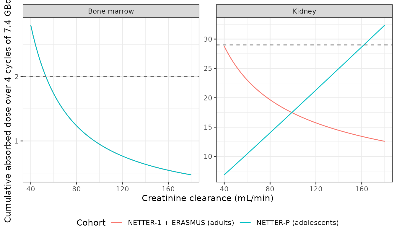
Replicates the mechanism behind Figure 7A of Sood 2026: in the pooled model the kidney absorbed dose FALLS with creatinine clearance in the adult studies and RISES with it in NETTER-P, because the study effect shifts the CrCL exponent from -0.55 to +1.03. Bone marrow carries no study effect and falls with CrCL in both cohorts.
The dashed lines are the 29 Gy kidney and 2 Gy bone-marrow thresholds. The adolescent kidney curve rising toward the threshold at high CrCL is a direct consequence of the +1.58 study term, and is the feature the paper itself flags as resting on ten patients.
Assumptions and deviations
Residual error encoded as exponential, not additive. Both the main text (“Constant residual error”, Tables 2 and 4) and the supplement (“additive (constant) error model was assumed”) name a constant error model. It is encoded here as
Cc ~ lnorm(expSd)– constant on the log-transformed observation – rather thanadd(addSd), because Figure 1 falsifies the linear-additive reading. The NETTER-1 prediction-corrected VPC spans 0.01-100 ng/mL with a roughly constant relative spread and its 90% prediction intervals still bracket a median near 0.05 ng/mL at 150 h. An additive residual SD of 0.40 ng/mL is eight-fold larger than that median, so roughly half of the simulated observations across the entire terminal phase would be negative and no log-axis VPC of that shape could be produced. The same argument applies to the adolescent model (SD 0.25 against a median near 0.06 ng/mL at 72 h in Figure 1B). The natural-log scale is corroborated by the width of the bands: a log10 reading of 0.25 would give a 5th-to-95th observed spread of about 6.5-fold in Figure 1B against the roughly 2.7-fold actually drawn.The peptide mass dose is not reported. The popPK dataset was built from the “actual mass dose” with blood radioactivity “converted to mass”, so the model’s clearances and volumes are mass-based and its observation is a mass concentration in ng/mL – but no mass is printed anywhere in the paper or supplement, and it is not recoverable from the 7.4 GBq activity because the cold peptide fraction of a vial grows as the 177Lu decays. The dose used in the cohort simulations here is calibrated from the paper’s own predicted median AUC(last) (Figure 5A) and lands near 196 ug for NETTER-1 and 247 ug for NETTER-P. This affects only the vignette’s simulations; the packaged models carry no dose.
The infusion duration is not reported either. It was back-solved from the dose-free ratio of the paper’s predicted median Cmax to its predicted median AUC(last) for the adults (7.3 / 36 = 0.2028 per h): a 1 h infusion reproduces 0.2029 per h, against 0.2255 for 30 min and 0.1666 for 2 h. Applying that same 1 h to the adolescent cohort – which was not used in the back-solve – reproduces 0.290 per h against the printed 0.277, so the assumption cross-validates. It is consistent with the Results noting one NETTER-1 patient as an outlier attributed to “rapid drug infusion (< 0.5 h)”, which implies the usual infusion is longer than half an hour.
The adult popPK demographics describe the wrong-sized set. Table 1 tabulates the n = 47 adult dosimetry population (NETTER-1 plus ERASMUS); the 20-patient popPK subset is never tabulated separately. The adult popPK model’s
populationmetadata records the n = 47 values with that caveat attached rather than leaving the fields empty.Kidney mass is not carried as a covariate column. It appears in Table 1 for both cohorts and was screened in both popPK covariate searches (and flagged by the adolescent stepwise search, at RSE 251.2), but it was retained in no final model and no coefficient is printed. It is recorded in the model files’
population$notesrather than proposed as a new canonical covariate.The four dosimetry outputs come from separate regressions. The supplement states that “As only one dosimetry value per subject was available, nonlinear regression (assuming proportional error) was performed for each organ separately”. Kidney and bone marrow are packaged as two outputs of one model file per dataset purely as a container: they share no parameter, no covariate coefficient and no random effect, so the joint representation is numerically identical to two independent fits.
Neither dosimetry model has a between-subject random effect. Each subject contributed one absorbed-dose value, so there is nothing to separate between-subject from residual variability; the proportional residual carries all unexplained variability. That is why the Supplemental Table 2 exceedance probabilities are a test of the residual SD.
The printed kidney
A_popis rounded.4.3in Table 3 is a one-decimal rounding of approximately 4.34, which is what produces the uniform 0.95% deficit against Supplemental Table 1 documented above. The packaged model carries the printed 4.3, per the policy of never tuning a parameter to match a validation target; the offset is uniform, quantified, and gated.The adolescent CrCL used to reproduce the pooled model’s 5.39 Gy is 121.4, not the Table 1 median of 122.1. Table 1’s median covers all 11 NETTER-P patients; the pooled dosimetry set carries only 10 of them, one having been excluded for unusable images. The 10-patient median is not printed, and 121.4 is the value that recovers the paper’s figure; 122.1 gives 5.42 Gy, 0.6% high.
Figure 5A’s NETTER-P predicted box disagrees with its own printed label. The panel prints
Med = 37.9under the adolescent predicted AUC(last) box, but the box itself is drawn spanning roughly 29-33.5 ng*h/mL with a median near 31.5 – about 20% below the label, while the other three boxes in that panel and all four in the Cmax panel agree with their labels. The printed label is used here, both because printed values outrank digitised ones and because it is the internally consistent reading: 10.5 / 37.9 = 0.277 per h against the model’s 0.290 on a 1 h infusion, whereas 10.5 / 31.5 = 0.333 per h would be 13% away in the opposite direction from the adult cohort. A reader wanting the adolescent mass dose should treat it as uncertain by at least that 20%.The study effect is a covariate on a covariate.
STUDY_NETTER_Pshifts the CrCL exponent in the kidney model rather than scaling the predicted dose, so it cannot be read as a percentage difference between cohorts. The paper itself flags the resulting sign reversal as provisional given n = 10 adolescents and the absence of renal impairment in that cohort.
Reference
- Sood M, Lachi Silva L, Ho YY, Blumenstein L, Cherfi A, Xu L, Khanshan F. [177Lu]Lu-DOTATATE population pharmacokinetics and dosimetry modeling for adolescent and adult patients with somatostatin receptor-positive gastroenteropancreatic neuroendocrine tumors. J Nucl Med. 2026;67(6):887-894. doi:10.2967/jnumed.125.270202