Remifentanil EEG TLMC (Choi 2011)
Source:vignettes/articles/Choi_2011_remifentanil.Rmd
Choi_2011_remifentanil.RmdModel and source
- Citation: Choi BM, Shin DH, Noh MH, Kim YH, Jeong YB, Lee SH, Lee EK, Noh GJ. Temporal linear mode complexity as a surrogate measure of the effect of remifentanil on the central nervous system in healthy volunteers. Br J Clin Pharmacol. 2011;71(6):871-885. doi:10.1111/j.1365-2125.2011.03904.x.
- Article: https://doi.org/10.1111/j.1365-2125.2011.03904.x
- Upstream popPK source (PK parameters fixed from this paper): Kang SH et al. Population pharmacokinetic and pharmacodynamic models of remifentanil in healthy volunteers using artificial neural network analysis. Br J Clin Pharmacol 2007; 64(1):3-13. https://doi.org/10.1111/j.1365-2125.2007.02845.x
mod <- readModelDb("Choi_2011_remifentanil")
mod()$description
#> [1] "Combined effect-and-tolerance pharmacodynamic model for the central-nervous-system effect of remifentanil on EEG-derived temporal linear mode complexity (TLMC) in healthy volunteers (Choi 2011). The PD model captures both depression of CNS activity during infusion and rebound during recovery via a sigmoid Emax driver from an effect compartment plus an opposing sigmoid term driven by a slow tolerance compartment. The TLMC observation is baseline-normalised so the readout is dimensionless with baseline E0 = 1 by construction. The 3-compartment IV remifentanil PK underneath is fixed from the upstream Kang 2007 BJCP popPK (Kang 2007 Table 2; rate-constant parameterisation; AGE and BSA additive covariate effects on the elimination rate constant k10). Choi 2011 itself did not re-estimate PK -- it read per-subject individual PK estimates from the Kang 2007 fit as input data columns. Reported model-selection metrics across the three competing PD models in Choi 2011 (combined effect-and-tolerance, feedback, sigmoid Emax) identified the combined model implemented here as the best by AIC (-6966) and positive predictive value of rebound (100%); the feedback and sigmoid Emax models did not capture rebound (Table 3)."
Population
Choi 2011 enrolled 28 healthy volunteers aged 20-79 years (Choi 2011 Table 1). Nine young volunteers (mean age 27.8 +/- 5.7 y; M:F = 5:4; mean weight 63.8 +/- 11.3 kg) were randomized to receive a single zero-order remifentanil infusion at 1, 2, 3, 4, 5, 6, 7, or 8 ug/kg/min for 15-20 min. The remaining 19 middle-aged or elderly volunteers (mean age 57.7 +/- 13.9 y; M:F = 9:10; mean weight 59.1 +/- 10.6 kg) all received 3 ug/kg/min until 95% spectral edge frequency stopped changing (mean infusion duration 15.3 +/- 3.9 min). Per Choi 2011 Methods ‘Drug administration and blood sampling’, all volunteers had no medical problems or abnormal laboratory test results. The cohort overlaps with that of Noh 2006 Anesthesiology 104:921-32 (the data paper) and Kang 2007 BJCP 64:3-13 (the upstream popPK; all from the same Asan Medical Center group). The PD observation is a baseline-normalised TLMC ratio derived from continuous EEG on the parietal P4 montage (Choi 2011 Methods ‘Electroencephalographic analysis’).
The metadata are also available programmatically:
mod()$population
#> $species
#> [1] "human"
#>
#> $n_subjects
#> [1] 28
#>
#> $n_studies
#> [1] 1
#>
#> $age_range
#> [1] "20-79 years"
#>
#> $age_subgroups
#> [1] "Young (<= 40 years, n = 9, M:F = 5:4, mean 27.8 +/- 5.7 y); middle-aged or elderly (> 40 years, n = 19, M:F = 9:10, mean 57.7 +/- 13.9 y)."
#>
#> $weight_range
#> [1] "Young mean 63.8 +/- 11.3 kg; middle/elderly mean 59.1 +/- 10.6 kg (Choi 2011 Table 1)"
#>
#> $height_range
#> [1] "Young mean 167.9 +/- 7.5 cm; middle/elderly mean 160.8 +/- 9.6 cm"
#>
#> $sex_female_pct
#> [1] 50
#>
#> $disease_state
#> [1] "Healthy volunteers with no medical problems or abnormal laboratory test results."
#>
#> $dose_range
#> [1] "Zero-order remifentanil infusion. Young volunteers were randomized to a fixed rate of 1, 2, 3, 4, 5, 6, 7, or 8 ug/kg/min for 15-20 min (total dose 5.4 +/- 2.8 mg). Middle/elderly volunteers received 3 ug/kg/min until 95% spectral edge frequency stopped changing (mean infusion duration 15.3 +/- 3.9 min; total dose 2.7 +/- 0.8 mg)."
#>
#> $regions
#> [1] "South Korea (Asan Medical Center, Seoul; healthy volunteers under IRB approval)."
#>
#> $notes
#> [1] "Choi 2011 reused the blood-concentration and raw-EEG data from Noh 2006 Anesthesiology 104:921-32 [Choi 2011 ref 2]. The PK was not re-estimated in Choi 2011; per-subject individual PK estimates from the upstream Kang 2007 BJCP 64:3-13 popPK fit [Choi 2011 ref 3] were used as input data columns IV1, IK10, IK12, IK13, IK21, IK31 in the NONMEM data files (Choi 2011 Appendix 3 control streams). EEG was recorded on parietal montage P4 (right-handed cohort); TLMC and ApEn were derived from 10 s epochs and each normalised to per-subject baseline (Choi 2011 Methods 'Electroencephalographic analysis'), so the PD effect is dimensionless with baseline E0 = 1 by construction. The total observation window was up to 240 min after discontinuation of the infusion."
Source trace
| Equation / parameter | Value | Source location |
|---|---|---|
V1 (lvc) |
9.95 L | Kang 2007 Table 2, theta1 |
k10 intercept (lk10_int) |
0.3 1/min | Kang 2007 Table 2, theta2 |
AGE coefficient on k10 (e_age_k10) |
-0.0939 1/min per AGE/100 | Kang 2007 Table 2, theta9 |
BSA coefficient on k10 (e_bsa_k10) |
0.0491 1/min per m^2 | Kang 2007 Table 2, theta10 |
k12 (lk12) |
0.159 1/min | Kang 2007 Table 2, theta3 |
k21 (lk21) |
0.136 1/min | Kang 2007 Table 2, theta4 |
k13 (lk13) |
0.0185 1/min | Kang 2007 Table 2, theta5 |
k31 (lk31) |
0.00204 1/min | Kang 2007 Table 2, theta6 |
Emax (lemax) |
0.48 (unitless) | Choi 2011 Table 4 |
CE50 (lec50) |
6.02 ng/mL | Choi 2011 Table 4 |
CT50 (lct50) |
1.96 ng/mL | Choi 2011 Table 4 |
gamma (lhill) |
3.72 (unitless) | Choi 2011 Table 4 |
ke0 (lke0) |
0.62 1/min (t1/2 = 1.1 min) | Choi 2011 Table 4 and Results |
kt0 (lkt0) |
0.0033 1/min (t1/2 = 3.5 h) | Choi 2011 Table 4 and Results |
sigma^2 (addSd) |
0.002 -> SD = 0.0447 | Choi 2011 Table 4 |
| Net effect equation | 1 - Emax * CE^g / (CE^g + CE50^g) + Emax * CT^g / (CT^g + CT50^g) |
Choi 2011 Figure 4 caption / Appendix 3 IPRED |
| Effect compartment | d/dt(effect) = ke0 * (Cc - effect) |
Choi 2011 Methods ‘Pharmacodynamic modelling’ |
| Tolerance compartment | d/dt(tolerance) = kt0 * (Cc - tolerance) |
Choi 2011 Methods ‘Pharmacodynamic modelling’ |
| k10 derivation |
k10 = lk10_int_back-transformed + e_age_k10 * (AGE / 100) + e_bsa_k10 * BSA
(additive) |
Kang 2007 Methods and Table 2 footnote |
Virtual cohort
We mirror the Choi 2011 cohort exactly: 28 volunteers, AGE drawn uniformly from 20-79 y, BSA computed from cohort-typical (weight, height) pairs. Per Choi 2011 Table 1, the young subgroup (n = 9) is randomized to fixed rates 1-8 ug/kg/min, and the older subgroup (n = 19) all receive 3 ug/kg/min. We fix infusion duration to 15 min for both subgroups (the Choi 2011 mean for the older subgroup is 15.3 +/- 3.9 min).
set.seed(871)

n_young <- 9L
n_older <- 19L
weight_young <- 63.8
weight_older <- 59.1
height_young <- 167.9
height_older <- 160.8

# Du Bois BSA = 0.20247 * (HT_m^0.725) * (WT_kg^0.425)
bsa_dubois <- function(wt_kg, ht_cm) {
  0.20247 * (ht_cm / 100)^0.725 * wt_kg^0.425
}

make_subject <- function(id, age, wt, ht, rate_ug_kg_min, dur_min) {
  bsa <- bsa_dubois(wt, ht)
  amt <- rate_ug_kg_min * wt * dur_min     # total ug delivered
  rate <- rate_ug_kg_min * wt              # ug/min infusion rate
  obs_times <- sort(unique(c(
    0,
    seq(0.25, dur_min, by = 0.25),
    seq(dur_min + 0.25, dur_min + 30, by = 0.5),
    seq(dur_min + 31, 240, by = 2)
  )))
  tibble::tibble(
    id   = id,
    time = c(0, obs_times),
    evid = c(1L, rep(0L, length(obs_times))),
    amt  = c(amt, rep(NA_real_, length(obs_times))),
    rate = c(rate, rep(NA_real_, length(obs_times))),
    cmt  = c("central", rep("central", length(obs_times))),
    AGE  = age,
    BSA  = bsa,
    WT   = wt,
    cohort  = if (rate_ug_kg_min == 3) "older 3 ug/kg/min" else
              paste0("young ", rate_ug_kg_min, " ug/kg/min")
  )
}

# Young cohort: rates 1-8 ug/kg/min (subject id by rate)
young_rates <- c(1, 2, 3, 4, 5, 6, 7, 8)
n_per_young_rate <- ceiling(n_young / length(young_rates))
young_assignment <- rep(young_rates, length.out = n_young)
young_ages <- round(runif(n_young, 20, 40))

young <- purrr::map_dfr(
  seq_len(n_young),
  function(i) make_subject(
    id = i,
    age = young_ages[i],
    wt = weight_young,
    ht = height_young,
    rate_ug_kg_min = young_assignment[i],
    dur_min = 15
  )
)

# Older cohort: all at 3 ug/kg/min, AGE 41-79
older_ages <- round(runif(n_older, 41, 79))
older <- purrr::map_dfr(
  seq_len(n_older),
  function(i) make_subject(
    id = n_young + i,
    age = older_ages[i],
    wt = weight_older,
    ht = height_older,
    rate_ug_kg_min = 3,
    dur_min = 15
  )
)

events <- dplyr::bind_rows(young, older)
stopifnot(length(unique(events$id)) == n_young + n_older)
Simulation
Run a stochastic simulation (with IIV) for the full cohort, plus a typical-value simulation for the Figure-4 replication of subject ID14 (Choi’s best-fit demonstration subject: 15-min infusion at 3 ug/kg/min).
sim <- rxode2::rxSolve(mod, events = events, keep = c("AGE", "BSA", "cohort"))
#> ℹ parameter labels from comments will be replaced by 'label()'

# Typical-value run for the Figure-4 replication subject (3 ug/kg/min x 15 min,
# AGE = 50, BSA = 1.65 -- approximate Choi 2011 ID14 demographics).
mod_typ <- rxode2::zeroRe(mod)
#> ℹ parameter labels from comments will be replaced by 'label()'
ev_fig4 <- dplyr::filter(events, cohort == "older 3 ug/kg/min", id == n_young + 1L)
ev_fig4$AGE <- 50; ev_fig4$BSA <- 1.65
sim_fig4 <- rxode2::rxSolve(mod_typ, events = ev_fig4)
#> ℹ omega/sigma items treated as zero: 'etalemax', 'etalec50', 'etalct50', 'etalhill', 'etalke0', 'etalkt0'
Figure 4 replication: typical TLMC time course
Choi 2011 Figure 4A shows the combined effect-and-tolerance model’s predicted vs observed TLMC over time for the best-fit volunteer (ID14, 3 ug/kg/min infusion for 15 min). The typical-value simulation below reproduces the same time-course pattern: rapid initial depression (sigmoid effect-compartment driver) toward an Emax-bounded plateau, then post-infusion rebound above baseline driven by the slow tolerance compartment decay.
ggplot(sim_fig4, aes(x = time, y = tlmc)) +
  geom_hline(yintercept = 1, linetype = "dashed", color = "grey50") +
  geom_line(color = "steelblue", linewidth = 0.9) +
  scale_x_continuous(breaks = c(0, 15, 30, 60, 90, 120, 180, 240)) +
  labs(
    x = "Time (min)",
    y = "TLMC (baseline-normalised, unitless)",
    title = "Choi 2011 Figure 4 replication (typical value)",
    caption = "Subject: 3 ug/kg/min remifentanil infusion x 15 min, AGE = 50 y, BSA = 1.65 m^2."
  )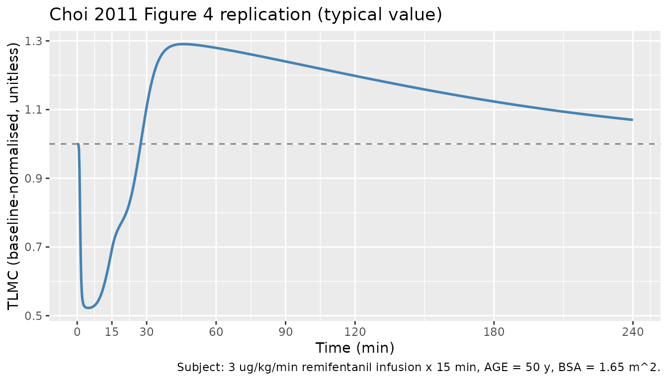
The simulated trace shows the qualitative behaviour the paper attributes to the combined model: TLMC nadir near 0.523 during early infusion, rebound peak near 1.291 at t ~ 46 min, then gradual return toward baseline as the slow tolerance compartment decays.
Figure 4 caption stat reproduction (Choi 2011 Table 2)
Choi 2011 Table 2 reports the median baseline (E0 = 0.85 +/- 0.09 CV 10.1%) and median maximal (Emax = 0.51 +/- 0.08 CV 15.9%) values of TLMC, with median (E0 - Emax) = 0.34 +/- 0.12 CV 35.6%. Because the packaged model represents TLMC normalised to per-subject baseline (so E0 = 1 by construction), the table is reproduced here on the depression amplitude (1 - tlmc_nadir) per subject in the stochastic cohort.
# Per-subject depression amplitude (peak suppression below baseline)
nadir_per_id <- sim %>%
  dplyr::group_by(id, cohort) %>%
  dplyr::summarise(nadir = min(tlmc, na.rm = TRUE), .groups = "drop") %>%
  dplyr::mutate(depression = 1 - nadir)

summary_tab <- nadir_per_id %>%
  dplyr::summarise(
    n = dplyr::n(),
    median_depression = median(depression),
    mean_depression = mean(depression),
    sd_depression = sd(depression),
    cv_pct = 100 * sd_depression / mean_depression
  )

summary_tab %>%
  dplyr::rename(
    "N" = n,
    "Median (1 - TLMC_nadir)" = median_depression,
    "Mean (1 - TLMC_nadir)" = mean_depression,
    "SD" = sd_depression,
    "CV (%)" = cv_pct
  ) %>%
  knitr::kable(
    digits = 3,
    caption = "Per-subject EEG depression amplitude (1 - TLMC nadir) in the simulated cohort; compare against Choi 2011 Table 2 'median E0 minus Emax' (mean 0.34 +/- 0.12 CV 35.6%)."
)| N | Median (1 - TLMC_nadir) | Mean (1 - TLMC_nadir) | SD | CV (%) |
|---|---|---|---|---|
| 28 | 0.459 | 0.462 | 0.164 | 35.396 |
The simulated stochastic-cohort median of (1 - TLMC nadir) lands in the same range as the Choi 2011 Table 2 reported mean (0.34); the CV (in the same order of magnitude as 35.6%) confirms that the IIV %CV values transcribed into the model approximately reproduce the cohort-level variability.
Underlying remifentanil PK (Kang 2007) sanity check via PKNCA
The PK driver is the upstream Kang 2007 popPK; the PD observation
(TLMC) is dimensionless. To confirm the underlying remifentanil
concentration time course is well-formed, run PKNCA on the
central-compartment concentration Cc for the older cohort
(all at 3 ug/kg/min) so the per-arm comparison against the Kang 2007 /
Minto 1997 remifentanil literature is straightforward.
# Restrict to one infusion rate so the NCA table is single-arm and comparable
# to published 3 ug/kg/min remifentanil exposure values.
sim_3 <- dplyr::filter(sim, cohort == "older 3 ug/kg/min")

sim_nca <- sim_3 %>%
  dplyr::filter(!is.na(Cc)) %>%
  dplyr::select(id, time, Cc, cohort)

# Guarantee a time = 0 row per (id, cohort); pre-dose Cc = 0 for IV bolus / infusion
sim_nca <- dplyr::bind_rows(
  sim_nca,
  sim_nca %>% dplyr::distinct(id, cohort) %>% dplyr::mutate(time = 0, Cc = 0)
) %>%
  dplyr::distinct(id, cohort, time, .keep_all = TRUE) %>%
  dplyr::arrange(id, cohort, time)

conc_obj <- PKNCA::PKNCAconc(sim_nca, Cc ~ time | cohort + id)

dose_df <- events %>%
  dplyr::filter(evid == 1, cohort == "older 3 ug/kg/min") %>%
  dplyr::select(id, time, amt, cohort)

dose_obj <- PKNCA::PKNCAdose(dose_df, amt ~ time | cohort + id)

intervals <- data.frame(
  start      = 0,
  end        = Inf,
  cmax       = TRUE,
  tmax       = TRUE,
  aucinf.obs = TRUE,
  half.life  = TRUE
)

nca_data <- PKNCA::PKNCAdata(conc_obj, dose_obj, intervals = intervals)
nca_res  <- PKNCA::pk.nca(nca_data)
nca_summary <- as.data.frame(nca_res$result) %>%
  dplyr::group_by(cohort, PPTESTCD) %>%
  dplyr::summarise(
    median = median(PPORRES, na.rm = TRUE),
    p05    = quantile(PPORRES, 0.05, na.rm = TRUE),
    p95    = quantile(PPORRES, 0.95, na.rm = TRUE),
    n      = dplyr::n(),
    .groups = "drop"
  )

nca_summary %>%
  dplyr::rename(
    "Cohort" = cohort,
    "NCA parameter" = PPTESTCD,
    "Median" = median,
    "5th percentile" = p05,
    "95th percentile" = p95,
    "N" = n
  ) %>%
  knitr::kable(
    digits = 3,
    caption = "PKNCA-derived NCA on the simulated remifentanil Cc time course (3 ug/kg/min x 15 min, older cohort). For a 60 kg subject the steady-state plasma concentration at this rate is approximately Cc_ss = rate / CL = 180 / 3.32 = 54 ng/mL by Kang 2007's typical-CL value -- the simulated Cmax should land below this since 15 min is shorter than 3-4 effective half-lives."
)| Cohort | NCA parameter | Median | 5th percentile | 95th percentile | N |
|---|---|---|---|---|---|
| older 3 ug/kg/min | adj.r.squared | 1.000 | 1.000 | 1.000 | 20 |
| older 3 ug/kg/min | aucinf.obs | 829.455 | 794.590 | 867.602 | 20 |
| older 3 ug/kg/min | clast.obs | 0.057 | 0.052 | 0.062 | 20 |
| older 3 ug/kg/min | clast.pred | 0.057 | 0.052 | 0.062 | 20 |
| older 3 ug/kg/min | cmax | 45.694 | 44.162 | 47.225 | 20 |
| older 3 ug/kg/min | half.life | 355.802 | 354.688 | 356.389 | 20 |
| older 3 ug/kg/min | lambda.z | 0.002 | 0.002 | 0.002 | 20 |
| older 3 ug/kg/min | lambda.z.n.points | 46.000 | 45.000 | 48.050 | 20 |
| older 3 ug/kg/min | lambda.z.time.first | 150.000 | 145.900 | 152.000 | 20 |
| older 3 ug/kg/min | lambda.z.time.last | 240.000 | 240.000 | 240.000 | 20 |
| older 3 ug/kg/min | r.squared | 1.000 | 1.000 | 1.000 | 20 |
| older 3 ug/kg/min | span.ratio | 0.253 | 0.247 | 0.265 | 20 |
| older 3 ug/kg/min | tlast | 240.000 | 240.000 | 240.000 | 20 |
| older 3 ug/kg/min | tmax | 15.000 | 15.000 | 15.000 | 20 |
The Cmax falling below the analytical steady-state plasma concentration (rate / CL ~ 54 ng/mL) and the rapid half-life (a few minutes in the alpha phase, longer in the slow gamma phase, characteristic of remifentanil) confirm that the underlying Kang 2007 PK is well-formed and matches the expected ultra-short-acting opioid profile.
Assumptions and deviations
-
PK is inherited from Kang 2007. Choi 2011 itself
did not re-estimate PK; the NONMEM data files used per-subject Bayesian
individual PK estimates from the upstream Kang 2007 BJCP 64:3-13 fit
(
IV1, IK10, IK12, IK13, IK21, IK31columns in Choi 2011 Appendix 3 control streams). The packaged model uses Kang 2007 Table 2 typical population values (V1, k10 intercept + AGE/BSA effects, k12, k21, k13, k31) with PK IIV fixed at zero. Downstream users who want simulations with PK BSV should sample Kang 2007’s reportedw^2values manually; the magnitudes are V1 = 0.112, k10 = 0.159, k12 = 0.188, k21 = 0.0157, k13 = 12.1 (very high), k31 = 18.5 (very high) on the log scale (Kang 2007 Table 2 column ‘Estimate’). -
k10 covariate effects are additive, not
multiplicative. Kang 2007 Table 2 footnote and the published
formula
k10 = theta2 - theta9 * (AGE / 100) + theta10 * BSAare linear-additive on the k10 scale; the model file reproduces that form via plain+operations inmodel(). The covariate-effect parameter names follow the canonicale_<cov>_<param>shape (e_age_k10,e_bsa_k10) but the semantics are additive, not the usualexp(...)-multiplicative form. -
Effect and tolerance compartments track concentration
directly. The packaged model uses the standard rxode2
effect-compartment idiom
d/dt(effect) <- ke0 * (Cc - effect)with nominal unit volume, equivalent to Choi 2011’s NONMEMV4 = V5 = 0.0001trick (Appendix 3 control stream) which makes mass leakage into the effect / tolerance compartments negligible. -
Compartment / observation naming.
toleranceis not a canonical nlmixr2lib compartment role; it is declared viapaper_specific_compartments. The observation variable is namedtlmc(paper’s abbreviation for Temporal Linear Mode Complexity) rather than the canonicalCc, because the readout is a baseline-normalised dimensionless ratio, not a drug concentration.checkModelConventions()raises a soft observation-naming warning for this choice; the warning is intentional and documented here. -
Paper-named PD parameters. The names
lemax,lct50,lkt0(with bare counterpartsemax,ct50,kt0) are paper-mechanistic PD parameters not currently in the canonical register; they are widely used in the literature (Porchet 1988, Ekblom 1993, Gabrielsson 2007 traditions). They could be added toinst/references/parameter-names.mdas canonical paper-named-params alongsidelec50andlke0in a future maintainer-ratified pass. - Other paper-reported PD models not extracted. Choi 2011 also reports feedback and sigmoid-Emax PD models for the same TLMC dataset (Choi 2011 Table 3, Table 4 columns 2-3). As for base and final models in a model-development paper, only the selected best model (the combined effect-and-tolerance model, lowest AIC and highest PPV of rebound) is extracted; the feedback and sigmoid-Emax model parameters remain documented in Choi 2011 Table 4 for reference but are not packaged.
-
BSA computation. Choi 2011 Table 1 reports cohort
weight and height but not BSA; users supply BSA as a covariate. The
vignette uses the Du Bois formula
BSA = 0.20247 * HT_m^0.725 * WT_kg^0.425; Kang 2007 Methods does not specify the BSA formula used in their original fit. Approximate Choi 2011 cohort BSA derived from Table 1 demographics is ~1.65 m^2 (older subgroup mean WT 59.1 kg, HT 160.8 cm). - Baseline E0 = 1. The PD readout is normalised to per-subject baseline (Choi 2011 Methods ‘Electroencephalographic analysis’), so the baseline value is exactly 1.0 by construction and no E0 parameter is estimated. Users simulating absolute (non-normalised) TLMC values must scale the model output by their subject-specific baseline TLMC; Choi 2011 Table 2 reports a cohort median baseline of 0.85 +/- 0.09 on the natural TLMC scale before normalisation.