Cefiderocol (Koenig 2025)
Source:vignettes/articles/Koenig_2025_cefiderocol.Rmd
Koenig_2025_cefiderocol.RmdModel and source
- Citation: Koenig C, Monogue ML, Shields RK, Sakon CM, Fratoni AJ, Roenfanz HF, Finklea JD, Pope JS, Nicolau DP, Kuti JL. Cefiderocol pharmacokinetics during acute pulmonary exacerbations in hospitalized adult persons with cystic fibrosis. Antimicrob Agents Chemother. 2025;69(1):e01539-24. doi:10.1128/aac.01539-24
- Description: Two-compartment population PK model for cefiderocol in hospitalized adults with cystic fibrosis during an acute pulmonary exacerbation, fitted nonparametrically with the Pmetrics NPAG algorithm and parameterised by clearance, central volume and the intercompartmental micro-rate constants k12 and k21
- Article: https://doi.org/10.1128/aac.01539-24 (PMC11784235; open access, CC BY)
- Supplement:
aac.01539-24-s0001.docx(APE criteria, Cockcroft-Gault formula, LC/MS-MS method, Figures S1-S3, the model-development AIC table and the covariance matrix of the final model)
Cefiderocol is a siderophore cephalosporin with activity against multidrug-resistant Gram-negative bacilli, including the Pseudomonas aeruginosa, Achromobacter spp. and Burkholderia cepacia complex isolates that drive acute pulmonary exacerbations (APE) in people with cystic fibrosis (pwCF). Koenig and colleagues report the first description of cefiderocol pharmacokinetics in adult pwCF hospitalized with an APE, fitting plasma concentrations nonparametrically with the adaptive grid (NPAG) algorithm in Pmetrics. The two-compartment disposition model they selected is the model packaged here.
The analysis was presented in preliminary form as poster P-1227 at
IDWeek 2024 (abstract ofae631.1409, Open Forum Infect Dis
2025;12(Suppl 1):S784). The poster’s parameter estimates differ from the
final publication’s and are superseded by them; see the Errata
section.
Population
Ten pwCF were enrolled in a prospective study across four United States sites; one was excluded for a positive pregnancy test before receiving study drug, so nine completed. Koenig 2025 Table 1 publishes every participant individually: mean age 33 years (SD 11, range 22-58), mean weight 62 kg (SD 10, range 45-78), mean height 170 cm (SD 7, range 157-180) and mean Cockcroft-Gault eGFR 117 mL/min (SD 24, range 71-164). Eight of nine were male. Six of nine were receiving CFTR modulator therapy during the study, which the Discussion proposes as the reason both renal clearance and protein binding resembled non-CF cohorts rather than the pre-modulator CF literature.
Every participant received 2 g of cefiderocol as a 3 h prolonged intravenous infusion, with the frequency set by the approved label according to eGFR: six received q8h and the three with augmented renal function (eGFR > 120 mL/min) received q6h. Sampling followed at least three prior doses, so all observations are at steady state, and was drawn at 0 (pre-dose), 1.5, 3, 3.25, 3.5, 4, 5, 6 and 8 h after the start of the final dose (80 samples in total).
Moderate-to-severe renal dysfunction (eGFR < 60 mL/min), any renal replacement therapy and haemodialysis were exclusion criteria, so this model carries no information about renal impairment, and the observed weight range is narrow. The Discussion cautions explicitly against extrapolating to pwCF of higher body weight or reduced eGFR.
knitr::kable(
  data.frame(
    Characteristic = c("Subjects", "Age (years)", "Weight (kg)", "Height (cm)",
                       "eGFR, Cockcroft-Gault (mL/min)", "Female", "CFTR modulator",
                       "Regimen", "Samples"),
    Value = c("9 (10 enrolled, 1 excluded)", "33 +/- 11 (22-58)",
              "62 +/- 10 (45-78)", "170 +/- 7 (157-180)", "117 +/- 24 (71-164)",
              "1 of 9", "6 of 9",
              "2 g over 3 h; q8h (n = 6) or q6h (n = 3) by eGFR", "80")
  ),
  caption = "Koenig 2025 Table 1 and Methods."
)| Characteristic | Value |
|---|---|
| Subjects | 9 (10 enrolled, 1 excluded) |
| Age (years) | 33 +/- 11 (22-58) |
| Weight (kg) | 62 +/- 10 (45-78) |
| Height (cm) | 170 +/- 7 (157-180) |
| eGFR, Cockcroft-Gault (mL/min) | 117 +/- 24 (71-164) |
| Female | 1 of 9 |
| CFTR modulator | 6 of 9 |
| Regimen | 2 g over 3 h; q8h (n = 6) or q6h (n = 3) by eGFR |
| Samples | 80 |
Source trace
Every ini() value and every model()
equation, with its location in the source.
knitr::kable(
  data.frame(
    Item = c("lcl", "lvc", "lk12", "lk21",
             "etalcl / etalvc / etalk12 / etalk21",
             "addSd", "propSd",
             "Two-compartment ODE structure",
             "q, vp", "Cc", "Cfree", "FU",
             "CRCL (excluded)", "WT (excluded)"),
    Value = c("log(5.66) L/h", "log(5.81) L", "log(4.29) 1/h", "log(2.25) 1/h",
              "0.05013 / 0.31306 / 0.50089 / 0.91615",
              "0.01224 mg/L", "0.10530",
              "central + peripheral1, micro-constants",
              "k12 * vc; q / k21", "central / vc", "FU * Cc",
              "1 - protein binding / 100",
              "slope 0.0399 L/h per mL/min, p = 0.0248",
              "slope 0.0427 L/kg, p = 0.764"),
    Source = c(rep("Table 2, population estimate (mean)", 4),
               "Table 2 SD column, via omega^2 = log(CV^2 + 1)",
               "Methods: C0 = 0.0068 x fitted gamma 1.8",
               "Methods: C1 = 0.0585 x fitted gamma 1.8",
               "Results: 'a two-compartment model (AIC 501) fitted the data better than a one-compartment model (AIC 548)'",
               "Algebraic identity of the Table 2 micro-constants",
               "Units declaration: dose mg, vc L",
               "Methods, individual target attainment analysis",
               "Table 3, protein binding column",
               "Supplement Figure S1 regression table; AIC table",
               "Supplement Figure S2 regression table")
  )
)| Item | Value | Source |
|---|---|---|
| lcl | log(5.66) L/h | Table 2, population estimate (mean) |
| lvc | log(5.81) L | Table 2, population estimate (mean) |
| lk12 | log(4.29) 1/h | Table 2, population estimate (mean) |
| lk21 | log(2.25) 1/h | Table 2, population estimate (mean) |
| etalcl / etalvc / etalk12 / etalk21 | 0.05013 / 0.31306 / 0.50089 / 0.91615 | Table 2 SD column, via omega^2 = log(CV^2 + 1) |
| addSd | 0.01224 mg/L | Methods: C0 = 0.0068 x fitted gamma 1.8 |
| propSd | 0.10530 | Methods: C1 = 0.0585 x fitted gamma 1.8 |
| Two-compartment ODE structure | central + peripheral1, micro-constants | Results: ‘a two-compartment model (AIC 501) fitted the data better than a one-compartment model (AIC 548)’ |
| q, vp | k12 * vc; q / k21 | Algebraic identity of the Table 2 micro-constants |
| Cc | central / vc | Units declaration: dose mg, vc L |
| Cfree | FU * Cc | Methods, individual target attainment analysis |
| FU | 1 - protein binding / 100 | Table 3, protein binding column |
| CRCL (excluded) | slope 0.0399 L/h per mL/min, p = 0.0248 | Supplement Figure S1 regression table; AIC table |
| WT (excluded) | slope 0.0427 L/kg, p = 0.764 | Supplement Figure S2 regression table |
Published individual estimates
Koenig 2025 publishes the maximum a posteriori (MAP) Bayesian parameter estimates for all nine participants (Table 2) together with each participant’s measured protein binding and simulated AUC24h (Table 3). That makes the paper unusually verifiable: the whole validation below is a deterministic reconstruction driven by the published per-subject parameters, with no random draws, so every check is reproducible on any machine and tight tolerances are appropriate.
subj <- data.frame(
  id        = c(1, 2, 3, 5, 6, 7, 4, 8, 9),
  regimen   = c(rep("2 g q8h", 6), rep("2 g q6h", 3)),
  tau       = c(rep(8, 6), rep(6, 3)),
  cl        = c(4.17, 4.01, 5.20, 5.13, 7.68, 5.37, 6.70, 5.03, 7.59),
  vc        = c(9.09, 5.60, 13.21, 6.05, 2.88, 2.25, 7.93, 2.41, 2.87),
  k12       = c(0.64, 7.11, 0.58, 0.50, 8.96, 4.72, 1.63, 4.82, 9.60),
  k21       = c(0.92, 9.95, 1.06, 0.50, 1.74, 1.15, 1.77, 1.30, 1.85),
  pb        = c(54, 45, 55, 47, 57, 56, 38, 49, 35),
  auc24_pub = c(1430, 1496, 1153, 1170, 781, 1117, 1194, 1590, 1054)
)
subj$FU <- 1 - subj$pb / 100

# The published population estimates are the arithmetic mean of these nine
# individual estimates, which confirms the Table 2 transcription.
chk_pop <- data.frame(
  Parameter = c("CL (L/h)", "Vc (L)", "k12 (1/h)", "k21 (1/h)"),
  Published = c(5.66, 5.81, 4.29, 2.25),
  `Mean of individuals` = round(
    c(mean(subj$cl), mean(subj$vc), mean(subj$k12), mean(subj$k21)), 3
  ),
  check.names = FALSE
)
knitr::kable(chk_pop)| Parameter | Published | Mean of individuals |
|---|---|---|
| CL (L/h) | 5.66 | 5.653 |
| Vc (L) | 5.81 | 5.810 |
| k12 (1/h) | 4.29 | 4.284 |
| k21 (1/h) | 2.25 | 2.249 |
Simulation of the published regimens
Each participant is simulated on their own regimen for four doses, which is the protocol Koenig 2025 used for its own target-attainment simulations (“profiles were generated for four doses to achieve steady state”), and evaluated over the final dosing interval.
mod <- rxode2::zeroRe(ui)

DOSE  <- 2000   # mg
DUR   <- 3      # h prolonged infusion
NDOSE <- 4
GRID  <- 0.05   # h

mkEvents <- function(d, grid = GRID) {
  do.call(rbind, lapply(seq_len(nrow(d)), function(i) {
    s <- d[i, ]
    dos <- data.frame(
      id = s$id, time = seq(0, (NDOSE - 1) * s$tau, by = s$tau),
      amt = DOSE, evid = 1, rate = DOSE / DUR, cmt = "central"
    )
    obs <- data.frame(
      id = s$id, time = seq(0, NDOSE * s$tau, by = grid),
      amt = NA_real_, evid = 0, rate = NA_real_, cmt = "central"
    )
    out <- rbind(dos, obs)
    out$FU <- s$FU
    out[order(out$time, -out$evid), ]
  }))
}

pars <- data.frame(
  id = subj$id, lcl = log(subj$cl), lvc = log(subj$vc),
  lk12 = log(subj$k12), lk21 = log(subj$k21)
)
sim <- rxode2::rxSolve(
  mod, params = pars, events = mkEvents(subj), returnType = "data.frame"
)
#> ℹ omega/sigma items treated as zero: 'etalcl', 'etalvc', 'etalk12', 'etalk21'
#> Warning: multi-subject simulation without without 'omega'
sim <- dplyr::left_join(
  sim, subj[, c("id", "regimen", "tau", "auc24_pub")], by = "id"
)
sim$ss_start <- (NDOSE - 1) * sim$tau
Structural check: the peripheral compartment is actually being solved
This is the load-bearing structural gate for this model, and it is
not decoration. rxode2 5.1.7 inspects an rxUi model for a
recognisable linear compartment parameterisation and, when it finds one,
replaces the d/dt() right-hand sides with its analytic
kernel. A version of this model that defined cl and
vc but not q and vp was
recognised as a one-compartment system, and the
peripheral compartment was silently discarded: peripheral1
vanished from the solve output and the concentration decayed
mono-exponentially at kel with no distribution phase.
Critically, an AUC-based check cannot detect this, because AUC over a dosing interval equals dose/CL for any linear model at steady state, so the collapsed model reproduces every published AUC24h exactly. The trough is what discriminates: under the correct two-compartment solve the lowest pre-dose concentration in the cohort is about 8 mg/L, whereas the collapsed one-compartment solve puts it at essentially zero.
trough <- sim %>%
  dplyr::filter(abs(time - NDOSE * tau) < 1e-9) %>%
  dplyr::transmute(id, regimen, Ctrough = Cc, Ctrough_free = Cfree)
knitr::kable(trough, digits = 2,
caption = "Steady-state trough at the end of the final interval.")| id | regimen | Ctrough | Ctrough_free |
|---|---|---|---|
| 1 | 2 g q8h | 25.07 | 11.53 |
| 2 | 2 g q8h | 15.44 | 8.49 |
| 3 | 2 g q8h | 21.44 | 9.65 |
| 5 | 2 g q8h | 11.88 | 6.30 |
| 6 | 2 g q8h | 8.32 | 3.58 |
| 7 | 2 g q8h | 11.03 | 4.85 |
| 4 | 2 g q6h | 20.57 | 12.75 |
| 8 | 2 g q6h | 26.68 | 13.60 |
| 9 | 2 g q6h | 18.62 | 12.10 |
stopifnot(
  # The peripheral state must survive into the solve.
  "peripheral1" %in% names(sim),
  # A genuine distribution phase. Realised minimum 8.32 mg/L; the collapsed
  # one-compartment solve gives < 0.01 mg/L, so this has a ~800-fold margin
  # and still goes red the moment the ODE is bypassed.
  min(trough$Ctrough) > 4
)
PKNCA validation
Noncompartmental analysis over the final dosing interval, grouped by regimen and participant.
sim_nca <- sim %>%
  dplyr::filter(time >= ss_start, !is.na(Cc)) %>%
  dplyr::select(id, regimen, time, Cc)

dose_df <- subj %>%
  dplyr::transmute(id, regimen, time = (NDOSE - 1) * tau, amt = DOSE)

intervals <- data.frame(
  regimen = c("2 g q8h", "2 g q6h"),
  start   = c(3 * 8, 3 * 6),
  end     = c(4 * 8, 4 * 6),
  cmax    = TRUE,
  cmin    = TRUE,
  tmax    = TRUE,
  auclast = TRUE,
  cav     = TRUE
)

nca_res <- PKNCA::pk.nca(PKNCA::PKNCAdata(
  PKNCA::PKNCAconc(sim_nca, Cc ~ time | regimen + id,
                   concu = "mg/L", timeu = "h"),
  PKNCA::PKNCAdose(dose_df, amt ~ time | regimen + id,
                   doseu = "mg", duration = DUR),
  intervals = intervals
))
nca <- as.data.frame(nca_res)
Per-participant AUC24h against Koenig 2025 Table 3
The interval AUC is scaled to 24 h (x 24/tau) to match the paper’s AUC24h.
auc <- nca %>%
  dplyr::filter(PPTESTCD == "auclast") %>%
  dplyr::transmute(id, regimen, auc_tau = PPORRES) %>%
  dplyr::left_join(subj[, c("id", "tau", "auc24_pub")], by = "id") %>%
  dplyr::mutate(
    auc24 = auc_tau * 24 / tau,
    pct   = 100 * (auc24 - auc24_pub) / auc24_pub
  ) %>%
  dplyr::arrange(id)

knitr::kable(
  auc %>%
    dplyr::transmute(
      id, regimen,
      `Published AUC24h (mg/L*h)` = auc24_pub,
      `Simulated AUC24h (mg/L*h)` = round(auc24, 1),
      `% diff` = round(pct, 2)
    ),
  caption = "Koenig 2025 Table 3, AUC24h column."
)| id | regimen | Published AUC24h (mg/L*h) | Simulated AUC24h (mg/L*h) | % diff |
|---|---|---|---|---|
| 1 | 2 g q8h | 1430 | 1437.9 | 0.55 |
| 2 | 2 g q8h | 1496 | 1496.2 | 0.02 |
| 3 | 2 g q8h | 1153 | 1152.9 | -0.01 |
| 4 | 2 g q6h | 1194 | 1193.8 | -0.01 |
| 5 | 2 g q8h | 1170 | 1169.4 | -0.05 |
| 6 | 2 g q8h | 781 | 781.2 | 0.03 |
| 7 | 2 g q8h | 1117 | 1117.2 | 0.02 |
| 8 | 2 g q6h | 1590 | 1589.9 | -0.01 |
| 9 | 2 g q6h | 1054 | 1053.7 | -0.03 |
sprintf("max |%% diff| in AUC24h: %.2f%%", max(abs(auc$pct)))
#> [1] "max |% diff| in AUC24h: 0.55%"
stopifnot(
  # Deterministic reconstruction, so this is tight by design. Realised 0.55%,
  # driven by subject 1 alone; the residual is the paper's own trapezoidal
  # integration of a 15-min grid, which slightly understates the peak, plus
  # rounding of CL to three significant figures. A mis-transcribed clearance,
  # dose or unit moves this by tens of percent.
  max(abs(auc$pct)) < 1.5
)
Group-mean AUC24h against the abstract and Results text
auc_group <- auc %>%
  dplyr::group_by(regimen) %>%
  dplyr::summarise(auclast = mean(auc24), .groups = "drop")

auc_ref <- data.frame(
  regimen = c("2 g q8h", "2 g q6h"),
  auclast = c(1191, 1279)   # Koenig 2025 Abstract and Table 3 "Mean" rows
)

cmp <- nlmixr2lib::ncaComparisonTable(
  auc_group, auc_ref,
  by     = "regimen",
  params = "auclast",
  units  = c(auclast = "mg/L*h, AUC24h at steady state")
)
knitr::kable(cmp, caption = attr(cmp, "footnote"))| NCA parameter | regimen | Reference | Simulated | % diff |
|---|---|---|---|---|
| AUClast (mg/L*h, AUC24h at steady state) | 2 g q8h | 1190 | 1190 | +0.1% |
| AUClast (mg/L*h, AUC24h at steady state) | 2 g q6h | 1280 | 1280 | +0.0% |
Per-participant %fT > MIC against Koenig 2025 Table 3
The paper evaluated free-drug time above the MIC on a 15-minute grid (“one data point every 15 min”). That discretisation is recoverable from the published values themselves: every q8h entry is an exact multiple of 1/32 (81% = 26/32, 69% = 22/32, 41% = 13/32) and every q6h entry an exact multiple of 1/24 (88% = 21/24, 92% = 22/24, 83% = 20/24). Reproducing the method exactly, rather than integrating a finer grid, therefore lets the 45 published cells be checked against their own arithmetic.
MICS <- c(2, 4, 8, 16, 32)

ftmic <- do.call(rbind, lapply(subj$id, function(i) {
  s <- subj[subj$id == i, ]
  grid15 <- seq((NDOSE - 1) * s$tau, NDOSE * s$tau - 0.25, by = 0.25)
  d <- sim[sim$id == i, ]
  cf <- stats::approx(d$time, d$Cfree, xout = grid15)$y
  data.frame(
    id = i, regimen = s$regimen, MIC = MICS,
    ft = vapply(MICS, function(m) 100 * mean(cf > m), numeric(1))
  )
}))

# Koenig 2025 Table 3, %fT > MIC block, transcribed per participant.
ftmic_pub <- data.frame(
  id  = rep(c(1, 2, 3, 5, 6, 7, 4, 8, 9), each = 5),
  MIC = rep(MICS, 9),
  ft_pub = c(100, 100, 100,  81, 34,
             100, 100, 100,  78, 50,
             100, 100, 100,  69, 16,
             100, 100,  88,  59, 38,
             100,  94,  69,  41,  0,
             100, 100,  81,  56, 22,
             100, 100, 100,  88, 46,
             100, 100, 100,  92, 54,
             100, 100, 100,  83, 42)
)

ftmic <- ftmic %>%
  dplyr::left_join(ftmic_pub, by = c("id", "MIC")) %>%
  dplyr::mutate(diff = ft - ft_pub)

# Guard against a silently empty comparison (pattern: all(logical(0)) is TRUE).
stopifnot(nrow(ftmic) == 45L, !anyNA(ftmic$ft_pub), !anyNA(ftmic$ft))

knitr::kable(
  ftmic %>%
    dplyr::mutate(cell = paste0(round(ft, 1), " / ", ft_pub)) %>%
    dplyr::select(id, regimen, MIC, cell) %>%
    tidyr::pivot_wider(names_from = MIC, values_from = cell,
                       names_prefix = "MIC "),
  caption = paste("Simulated / published %fT > MIC per participant",
                  "(Koenig 2025 Table 3).")
)| id | regimen | MIC 2 | MIC 4 | MIC 8 | MIC 16 | MIC 32 |
|---|---|---|---|---|---|---|
| 1 | 2 g q8h | 100 / 100 | 100 / 100 | 100 / 100 | 81.2 / 81 | 34.4 / 34 |
| 2 | 2 g q8h | 100 / 100 | 100 / 100 | 100 / 100 | 78.1 / 78 | 50 / 50 |
| 3 | 2 g q8h | 100 / 100 | 100 / 100 | 100 / 100 | 68.8 / 69 | 15.6 / 16 |
| 5 | 2 g q8h | 100 / 100 | 100 / 100 | 87.5 / 88 | 59.4 / 59 | 37.5 / 38 |
| 6 | 2 g q8h | 100 / 100 | 93.8 / 94 | 68.8 / 69 | 40.6 / 41 | 0 / 0 |
| 7 | 2 g q8h | 100 / 100 | 100 / 100 | 81.2 / 81 | 56.2 / 56 | 21.9 / 22 |
| 4 | 2 g q6h | 100 / 100 | 100 / 100 | 100 / 100 | 87.5 / 88 | 45.8 / 46 |
| 8 | 2 g q6h | 100 / 100 | 100 / 100 | 100 / 100 | 91.7 / 92 | 54.2 / 54 |
| 9 | 2 g q6h | 100 / 100 | 100 / 100 | 100 / 100 | 83.3 / 83 | 41.7 / 42 |
sprintf("max |difference| across %d cells: %.2f percentage points",
        nrow(ftmic), max(abs(ftmic$diff)))
#> [1] "max |difference| across 45 cells: 0.50 percentage points"
sprintf("cells reproduced exactly: %d of %d",
        sum(abs(ftmic$diff) < 1e-9), nrow(ftmic))
#> [1] "cells reproduced exactly: 25 of 45"
stopifnot(
  # Deterministic. Realised 0.5 pp, which is exactly the paper's rounding of
  # its own n/32 and n/24 grid fractions to whole percent, so 1 pp is the
  # tightest bound that is arithmetically achievable here.
  max(abs(ftmic$diff)) <= 1
)
The group means also reproduce the Abstract and Results narrative: at MICs of 4, 8 and 16 mg/L the q8h arm attains a mean %fT > MIC that the paper reports as 99%, 90% and 64%, and the q6h arm 100%, 100% and 87%.
ftmic_group <- ftmic %>%
  dplyr::group_by(regimen, MIC) %>%
  dplyr::summarise(simulated = mean(ft), published = mean(ft_pub),
                   .groups = "drop") %>%
  dplyr::mutate(dplyr::across(c(simulated, published), ~ round(.x, 1)))
knitr::kable(
  ftmic_group %>%
    dplyr::rename("Simulated mean %fT > MIC" = simulated,
                  "Published mean %fT > MIC" = published),
  caption = "Group means, Koenig 2025 Table 3 'Mean' rows."
)| regimen | MIC | Simulated mean %fT > MIC | Published mean %fT > MIC |
|---|---|---|---|
| 2 g q6h | 2 | 100.0 | 100.0 |
| 2 g q6h | 4 | 100.0 | 100.0 |
| 2 g q6h | 8 | 100.0 | 100.0 |
| 2 g q6h | 16 | 87.5 | 87.7 |
| 2 g q6h | 32 | 47.2 | 47.3 |
| 2 g q8h | 2 | 100.0 | 100.0 |
| 2 g q8h | 4 | 99.0 | 99.0 |
| 2 g q8h | 8 | 89.6 | 89.7 |
| 2 g q8h | 16 | 64.1 | 64.0 |
| 2 g q8h | 32 | 26.6 | 26.7 |
Replicating the published figures
Individual steady-state profiles (Figure S3)
prof <- sim %>%
  dplyr::filter(time >= ss_start) %>%
  dplyr::mutate(t_rel = time - ss_start)

ggplot2::ggplot(prof, ggplot2::aes(t_rel, Cc, group = id, colour = regimen)) +
  ggplot2::geom_line() +
  ggplot2::labs(
    x = "Time after start of the final infusion (h)",
    y = "Total plasma cefiderocol (mg/L)", colour = NULL,
    title = "Steady-state profiles from the published individual estimates",
    subtitle = "Replicates the shape of Koenig 2025 Figure S3"
  ) +
  ggplot2::theme_bw() +
  ggplot2::theme(legend.position = "bottom")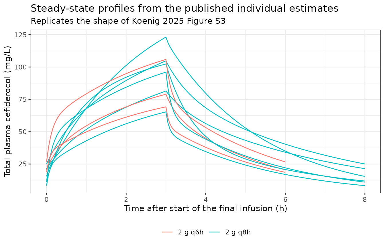
AUC24h in pwCF against the phase III trials (Figure 2)
Koenig 2025 Figure 2 compares steady-state AUC24h in pwCF with the phase III cUTI and HABP/VABP populations. The Discussion supplies the comparator values: cUTI 1944 (SD 1097) and HABP/VABP 1773 (SD 1503) mg/Lh. The paper’s point is that pwCF exposures are lower*, which it attributes to the deliberately narrow eGFR range studied here (71-164 mL/min) against 7-540 mL/min in the phase III trials, which enrolled patients with renal dysfunction.
ggplot2::ggplot(auc, ggplot2::aes(regimen, auc24)) +
  ggplot2::geom_boxplot(width = 0.4, outlier.shape = NA) +
  ggplot2::geom_jitter(width = 0.08, height = 0, size = 2) +
  ggplot2::geom_hline(yintercept = 1944, linetype = "dashed") +
  ggplot2::geom_hline(yintercept = 1773, linetype = "dotted") +
  ggplot2::annotate("text", x = 0.6, y = 1944, vjust = -0.5, size = 3,
                    label = "cUTI mean 1944") +
  ggplot2::annotate("text", x = 0.6, y = 1773, vjust = 1.4, size = 3,
                    label = "HABP/VABP mean 1773") +
  ggplot2::labs(x = NULL, y = "Steady-state AUC24h (mg/L*h)",
                title = "pwCF exposures against the phase III comparators",
                subtitle = "Replicates Koenig 2025 Figure 2") +
  ggplot2::theme_bw()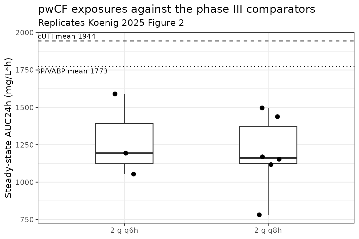
Interindividual variability
The packaged ini() carries the Table 2 SD column as
lognormal variances. Two consequences are worth making explicit, because
both are visible in a simulated cohort.
cohort_arm <- function(regimen, tau, n = 100, seed = 20250124) {
  # Re-seed inside the loop so the two arms share common random numbers.
  rxode2::rxSetSeed(seed)
  set.seed(seed)
  d <- data.frame(
    id = seq_len(n), regimen = regimen, tau = tau,
    # FU is a measured per-subject input; resampled from the nine observed
    # values, since the paper reports no distribution for it.
    FU = sample(subj$FU, n, replace = TRUE)
  )
  s <- rxode2::rxSolve(ui, events = mkEvents(d, grid = 0.25),
                       returnType = "data.frame")
  s$regimen <- regimen
  s$tau <- tau
  s
}
cohort <- rbind(cohort_arm("2 g q8h", 8), cohort_arm("2 g q6h", 6))

cohort_summary <- cohort %>%
  dplyr::distinct(regimen, id, cl, vc, k12, k21) %>%
  dplyr::group_by(regimen) %>%
  dplyr::summarise(
    n = dplyr::n(),
    `median CL` = round(median(cl), 2),
    `mean CL`   = round(mean(cl), 2),
    `median Vc` = round(median(vc), 2),
    .groups = "drop"
  )
knitr::kable(cohort_summary,
caption = "Simulated cohort, 100 participants per arm.")| regimen | n | median CL | mean CL | median Vc |
|---|---|---|---|---|
| 2 g q6h | 100 | 5.62 | 5.67 | 5.44 |
| 2 g q8h | 100 | 5.62 | 5.67 | 5.44 |
ggplot2::ggplot(
  cohort %>% dplyr::filter(time >= (NDOSE - 1) * tau) %>%
    dplyr::mutate(t_rel = time - (NDOSE - 1) * tau),
  ggplot2::aes(t_rel, Cc, group = id)
) +
  ggplot2::geom_line(alpha = 0.12) +
  ggplot2::facet_wrap(~ regimen) +
  ggplot2::scale_y_log10() +
  ggplot2::labs(x = "Time after start of the final infusion (h)",
                y = "Total plasma cefiderocol (mg/L)",
                title = "Steady-state variability implied by the Table 2 SDs") +
  ggplot2::theme_bw()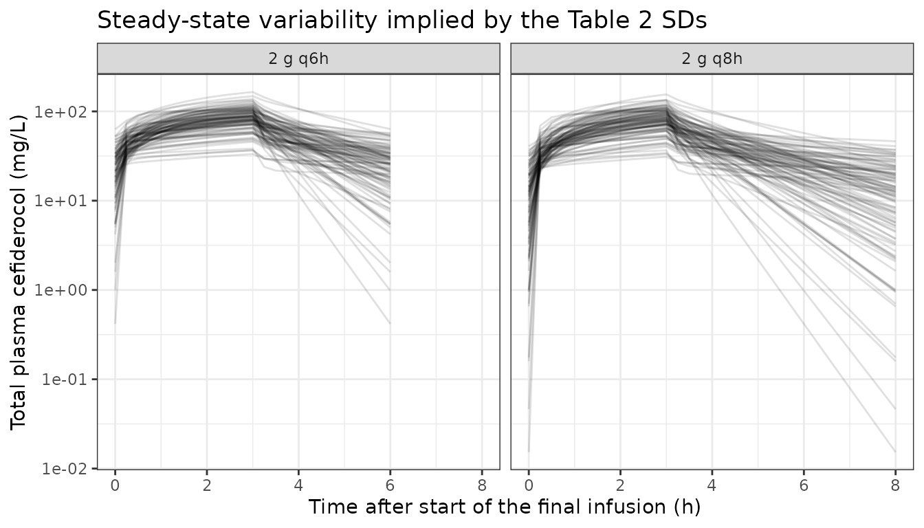
First, because the published central estimates are encoded as
lognormal medians while the paper reports arithmetic
means, a simulated cohort’s mean sits above the published value
by a factor of exp(omega^2 / 2):
om2 <- c(cl = 0.05013, vc = 0.31306, k12 = 0.50089, k21 = 0.91615)
knitr::kable(
  data.frame(
    Parameter = names(om2),
    `Published mean` = c(5.66, 5.81, 4.29, 2.25),
    `Encoded median` = c(5.66, 5.81, 4.29, 2.25),
    `Implied cohort mean` = round(c(5.66, 5.81, 4.29, 2.25) * exp(om2 / 2), 2),
    `Offset (%)` = round(100 * (exp(om2 / 2) - 1), 1),
    check.names = FALSE
  ),
  caption = "Consequence of encoding a reported mean as a lognormal median."
)| Parameter | Published mean | Encoded median | Implied cohort mean | Offset (%) | |
|---|---|---|---|---|---|
| cl | cl | 5.66 | 5.66 | 5.80 | 2.5 |
| vc | vc | 5.81 | 5.81 | 6.79 | 16.9 |
| k12 | k12 | 4.29 | 4.29 | 5.51 | 28.5 |
| k21 | k21 | 2.25 | 2.25 | 3.56 | 58.1 |
Second, the encoded variances come from the diagonal of the
supplement covariance matrix rather than from the Table 2 SD column,
because the matrix carries the unrounded variances while Table 2 rounds
their square roots to three significant figures. The check below pins
both halves of that claim: the encoded omega^2 values are
exactly log(1 + var/mean^2) from the matrix diagonal, and
the matrix diagonal reproduces the printed SDs to their stated
precision.
means      <- c(cl = 5.66, vc = 5.81, k12 = 4.29, k21 = 2.25)
cov_diag   <- c(cl = 1.647, vc = 12.409, k12 = 11.966, k21 = 7.592)
printed_sd <- c(cl = 1.28, vc = 3.52, k12 = 3.46, k21 = 2.76)
implied    <- log(1 + cov_diag / means^2)

cv_chk <- data.frame(
  Parameter = names(om2),
  `Table 2 SD` = printed_sd,
  `sqrt(diag(cov))` = round(sqrt(cov_diag), 3),
  `Encoded omega^2` = om2,
  `omega^2 from cov` = round(implied, 5),
  `Encoded CV (%)` = round(100 * sqrt(exp(om2) - 1), 1),
  check.names = FALSE
)
knitr::kable(cv_chk, row.names = FALSE)| Parameter | Table 2 SD | sqrt(diag(cov)) | Encoded omega^2 | omega^2 from cov | Encoded CV (%) |
|---|---|---|---|---|---|
| cl | 1.28 | 1.283 | 0.05013 | 0.05013 | 22.7 |
| vc | 3.52 | 3.523 | 0.31306 | 0.31306 | 60.6 |
| k12 | 3.46 | 3.459 | 0.50089 | 0.50089 | 80.6 |
| k21 | 2.76 | 2.755 | 0.91615 | 0.91615 | 122.5 |
Assumptions and deviations
The published estimates are arithmetic means, encoded as lognormal medians. Koenig 2025 Table 2 reports “Population estimate (mean +/- SD)”, and each value is the mean of the nine published individual MAP estimates (verified above). They are encoded as
log(mean), following the convention used for the other nonparametric (NPAG) models in this library, so that a typical-value simulation returns the published number. The medians of the nine individual estimates are lower (CL 5.20, Vc 5.60, k12 4.72, k21 1.30); a user who wants the cohort mean to match the paper should subtractomega^2 / 2from eachl-parameter.-
The published covariance matrix is not transferable to a lognormal block, so the etas are independent. The supplement publishes the full 4x4 covariance matrix of the nonparametric joint density, and its
sqrt(diag)reproduces all four Table 2 SDs to three significant figures, so it is certainly the matrix behind Table 2:CL Vc k12 k21 CL 1.647 Vc -1.586 12.409 k12 2.322 -8.819 11.966 k21 -1.184 -0.704 3.721 7.592 It cannot be carried over, because no multivariate lognormal has these means and this covariance. The implied Vc-k12 correlation is -0.724, but at these CVs (60.6% and 80.6%) the lognormal-feasible range for that pair is only -0.669 to 0.994. The moment-matched log-scale matrix is therefore indefinite (smallest eigenvalue -0.085) and
chol()fails on it, which would abort every stochastic solve. The other five pairs are individually feasible, but a block OMEGA must be jointly positive definite, so the diagonal is the only faithful option. The matrix is reproduced here so a user can apply their own nearest-positive-definite projection if they want the correlation structure. The residual error folds the fitted gamma into the assay polynomial. Pmetrics weights observations by an assay SD polynomial
C0 + C1*[obs] + C2*[obs]^2 + C3*[obs]^3scaled by a fitted gamma. Koenig 2025 gives C0 = 0.0068, C1 = 0.0585, C2 = C3 = 0 and a fitted gamma of 1.8, so the encoded SD is1.8 * (0.0068 + 0.0585 * Cc). Because C2 = C3 = 0 the polynomial is linear in the observation, which iscombined1()(a direct sum) and not nlmixr2’s default quadrature combination. The two terms are left estimable rather thanfixed()because, although C0 and C1 are stated assay constants, the gamma multiplying both of them was fitted.Vp and Q are derived, not estimated. The paper’s parameterisation is CL, Vc, k12 and k21, so the peripheral volume is identified only implicitly as
Vp = Vc * k12 / k21(11.1 L at the population estimates, with Q = 24.9 L/h). Definingqandvpinmodel()is also required for rxode2 5.1.7 to solve the two-compartment system at all – see the structural check above.The final model has no covariates. eGFR was the one significant correlate of clearance (supplement Figure S1: slope 0.0399 L/h per mL/min, p = 0.0248) but no eGFR model reduced the AIC by more than 2, and body weight was not significant for Vc (p = 0.764). Both are recorded in
covariatesDataExcludedwith their regression statistics rather than being silently dropped. Because eGFR < 60 mL/min was an exclusion criterion, the model must not be used to predict renal impairment.FUis measured data, converted from the reported protein binding. Koenig 2025 reports protein binding, soFU = 1 - PB/100; the Table 3 per-subject values give FU 0.43-0.65 (mean 0.52).FUscales only the free concentrationCfreethat drives target attainment; it does not scale any disposition parameter. In the simulated cohort above,FUis resampled from the nine measured values because the paper reports no distribution for it.The Methods protein-binding formula is missing a bracket. It is printed as
protein binding [%] = 1 - CPFF/CPlasma * 100, which is dimensionally inconsistent; it means(1 - CPFF/CPlasma) * 100, as the Table 3 values between 35 and 57 confirm.The cohort simulation is illustrative, not a VPC. The paper publishes no observed concentrations, so there is nothing to overlay; the cohort exists only to show the spread implied by the Table 2 SDs. Its assertions are deliberately structural (arm sizes) rather than numeric, because a cohort-derived statistic is not reproducible across solver thread counts.
Errata and provenance notes
-
The IDWeek 2024 poster is superseded. This analysis was first presented as poster P-1227 (abstract
ofae631.1409, Open Forum Infect Dis 2025;12(Suppl 1):S784), whose estimates differ materially from the final paper’s. The peer-reviewed values are used throughout; the poster’s are recorded here only so that a reader who finds the abstract first can tell the two apart.Quantity Poster P-1227 Final paper CL (L/h) 5.69 +/- 1.45 5.66 +/- 1.28 Vc (L) 7.42 +/- 3.74 5.81 +/- 3.52 k12 (1/h) 2.54 +/- 1.76 4.29 +/- 3.46 k21 (1/h) 2.72 +/- 3.04 2.25 +/- 2.76 Protein binding 45% (38-51) 48% (35-57) AIC, 2-compartment 514 501 AUC24h, q8h 1210 (790-1460) 1191 (781-1496) AUC24h, q6h 1241 (950-1578) 1279 (1054-1590) The poster also describes renal dosing by “creatinine clearance (CrCL) by Cockroft-Gault” while the paper says “estimated glomerular filtration rate (eGFR) … by Cockcroft-Gault”. These are the same quantity under two names; the supplement’s formula is the standard Cockcroft-Gault creatinine clearance, computed on ideal (or adjusted) body weight.
The supplement’s table captions are offset by one. In
aac.01539-24-s0001.docxthe caption “Table S1: Performance of tested models” is attached to the Figure S1 eGFR-versus-CL regression table, and “Table S2: Covariance matrix …” to the Figure S2 weight-versus-Vc regression table. The captioned content actually appears in the two unlabelled tables that follow, under the headings “Model development process” and “Covariance Matrix of final pharmacokinetic model”. Values in this vignette are taken from the content, not the captions.The eGFR regression slope is quoted twice with different precision. The Discussion says “the slope (0.039)”; the supplement regression table gives 0.0399. The tabulated value is used.
Subject numbering in Table 3 is not sequential. Table 3 lists the six q8h participants (IDs 1, 2, 3, 5, 6, 7) before the three q6h participants (IDs 4, 8, 9), whereas Tables 1 and 2 run 1 through 9. The join above is by participant ID, not row order.