Onset of nonlinear PK for mavrilimumab, efalizumab, romosozumab (Stein 2018)
Source:vignettes/articles/Stein_2018_mAb_nonlinear_PK.Rmd
Stein_2018_mAb_nonlinear_PK.RmdModel and source
- Citation: Stein AM, Peletier LA. Predicting the onset of nonlinear pharmacokinetics. CPT Pharmacometrics Syst Pharmacol. 2018 Oct;7(10):670-677.
- Article: https://doi.org/10.1002/psp4.12316
- Underlying data sources:
- Mavrilimumab (anti-GM-CSF receptor): Burmester GR, et al. Ann Rheum Dis. 2011;70(9):1542-1549.
- Efalizumab (anti-CD11a): Bauer RJ, et al. J Pharmacokinet Biopharm. 1999;27(4):397-420.
- Romosozumab (anti-sclerostin): Padhi D, et al. J Bone Miner Res. 2011;26(1):19-26.
Stein and Peletier (2018) derive an analytical expression for the
critical concentration Ccrit at which the elimination rate
of a monoclonal antibody with combined linear plus saturable
(target-mediated) clearance doubles, marking the transition between
approximately-linear and nonlinear PK. They fit two-compartment
quasi-steady-state (QSS) TMDD models to the published PK data of three
antibodies (mavrilimumab, efalizumab, romosozumab) and use those
typical-value fits to illustrate how
Ccrit = Vmax / CL = ksyn / (CL/Vc) lines up with the
visible kink in the concentration-time curves.
This vignette covers all three drugs because they share a paper, a
structural model, and a single narrative. The packaged models live in
three companion files under
inst/modeldb/specificDrugs/:
data.frame(
  Drug   = c("Mavrilimumab", "Efalizumab", "Romosozumab"),
  Target = c("GM-CSF receptor alpha", "CD11a (LFA-1)", "Sclerostin"),
  Model  = c("Stein_2018_mavrilimumab",
             "Stein_2018_efalizumab",
             "Stein_2018_romosozumab")
) |> knitr::kable()| Drug | Target | Model |
|---|---|---|
| Mavrilimumab | GM-CSF receptor alpha | Stein_2018_mavrilimumab |
| Efalizumab | CD11a (LFA-1) | Stein_2018_efalizumab |
| Romosozumab | Sclerostin | Stein_2018_romosozumab |
Population
The packaged parameters in Stein and Peletier 2018 Table 1 are typical-value fits to phase 1 / early-phase PK data from three previously published trials:
- Mavrilimumab (Burmester 2011) – adults with rheumatoid arthritis; single IV doses ranging from 0.01 to 10 mg/kg.
- Efalizumab (Bauer 1999) – adults with psoriasis; single IV doses ranging from 0.03 to 10 mg/kg.
- Romosozumab (Padhi 2011) – healthy adults; single IV doses including 1, 5, and 10 mg/kg.
Stein and Peletier 2018 (Methods, Model analysis, fitting, and
simulation) note that they fixed ke(R) = ke(CR) in all
three fits, an assumption commonly made for membrane-bound targets where
ke(R) is poorly identified from PK alone. The article
(Model fit section, page 672) additionally cautions that the large
values for ke(R) and ke(CR) reported for
efalizumab (4400/day) and romosozumab (860/day) reflect the
practical unidentifiability of these parameters in that
experimental setting – they are not meant as physiological
estimates.
The article does not report between-subject variability or residual
error for the fits; the packaged models are therefore typical-value only
and have no IIV or residual error structure. Programmatically, the
per-model population is available via
readModelDb("<model>")$population.
Source trace
Every parameter is taken directly from Stein and Peletier 2018 Table 1. The structural model is paper Eq. 7 with the QSS algebraic relations from paper Eq. 5.
| Drug | Parameter | Value (Table 1) | Units |
|---|---|---|---|
| Mavrilimumab | Vc | 2.8 | L |
| Mavrilimumab | Vp | 5.6 | L |
| Mavrilimumab | CL | 0.3 | L/day |
| Mavrilimumab | Q | 1.7 | L/day |
| Mavrilimumab | ksyn | 2.4 | nM/day |
| Mavrilimumab | Kss | 1.1 | nM |
| Mavrilimumab | ke(R) | 2.2 | 1/day |
| Mavrilimumab | ke(CR) | 2.2 | 1/day |
| Efalizumab | Vc | 2.4 | L |
| Efalizumab | Vp | 3.6 | L |
| Efalizumab | CL | 0.46 | L/day |
| Efalizumab | Q | 9.7 | L/day |
| Efalizumab | ksyn | 8.5 | nM/day |
| Efalizumab | Kss | 1.2 | nM |
| Efalizumab | ke(R) | 4400 | 1/day |
| Efalizumab | ke(CR) | 4400 | 1/day |
| Romosozumab | Vc | 2.4 | L |
| Romosozumab | Vp | 2.6 | L |
| Romosozumab | CL | 0.25 | L/day |
| Romosozumab | Q | 0.54 | L/day |
| Romosozumab | ksyn | 6.1 | nM/day |
| Romosozumab | Kss | 12 | nM |
| Romosozumab | ke(R) | 860 | 1/day |
| Romosozumab | ke(CR) | 860 | 1/day |
| Equation | Source |
|---|---|
| Two-compartment QSS TMDD ODE | Stein and Peletier 2018 Eq. 7 |
| QSS algebraic relations | Stein and Peletier 2018 Eq. 5 |
| Critical concentration Ccrit | Stein and Peletier 2018 Eq. 14 |
Critical concentration
The closed-form expression for Ccrit in the
two-compartment QSS TMDD model (Stein and Peletier 2018 Eq. 14, derived
under the rapid-exchange limit Q >> CL and
Q >> Vmax) is
Ccrit = Vmax / CL = ksyn * Vc / CLSubstituting the Table 1 values directly gives a per-drug
Ccrit:
mav <- rxode2::rxode2(readModelDb("Stein_2018_mavrilimumab"))
efa <- rxode2::rxode2(readModelDb("Stein_2018_efalizumab"))
rom <- rxode2::rxode2(readModelDb("Stein_2018_romosozumab"))

ccrit_nM <- function(mod) {
  ini  <- as.data.frame(mod$iniDf)
  vc   <- exp(ini$est[ini$name == "lvc"])
  cl   <- exp(ini$est[ini$name == "lcl"])
  ksyn <- exp(ini$est[ini$name == "lksyn"])
  ksyn * vc / cl
}

ccrit_tbl <- tibble::tibble(
  Drug      = c("Mavrilimumab", "Efalizumab", "Romosozumab"),
  Ccrit_nM  = c(ccrit_nM(mav), ccrit_nM(efa), ccrit_nM(rom)),
  Ccrit_ug_per_mL = Ccrit_nM * 150e3 / 1e9 * 1e3  # nM -> ug/mL using 150 kDa MW
)
knitr::kable(ccrit_tbl, digits = 2,
caption = "Critical concentration computed from Stein and Peletier 2018 Eq. 14 using Table 1 parameters. The 150 kDa molecular weight follows Stein and Peletier 2018 page 672.")| Drug | Ccrit_nM | Ccrit_ug_per_mL |
|---|---|---|
| Mavrilimumab | 22.40 | 3.36 |
| Efalizumab | 44.35 | 6.65 |
| Romosozumab | 58.56 | 8.78 |
Simulation: replicate Figure 1
Figure 1 of Stein and Peletier 2018 shows model predictions for each
drug across a range of single IV bolus doses (mg/kg). The dot-marked
Ccrit line is overlaid to highlight the transition between
linear and nonlinear elimination.
We simulate each drug at a common set of single IV doses (0.1, 0.3,
1, 3, 10 mg/kg) using the packaged Stein_2018_<drug>
models. The molar dose conversion follows Stein and Peletier 2018 page
672:
dose_nmol = dose_mg_per_kg * 70 kg / 150 kDa * 1e9 nmol/mol
mg_kg_to_nmol <- function(mg_per_kg) mg_per_kg * 70 / 150e3 * 1e9
nM_to_ug_per_mL <- function(conc_nM) conc_nM * 150e3 / 1e9 * 1e3

dose_levels_mg_kg <- c(0.1, 0.3, 1, 3, 10)

# Observation grid: dense early to capture the bolus peak, then daily out to 3
# months (Figure 1 x-axis: 0-3 months).
obs_times <- sort(unique(c(
  seq(0, 1, by = 0.05),
  seq(1, 7, by = 0.25),
  seq(7, 90, by = 0.5)
)))

build_events <- function(drug_label, model_name, doses_mg_kg) {
  out <- vector("list", length(doses_mg_kg))
  for (i in seq_along(doses_mg_kg)) {
    d_mg_kg <- doses_mg_kg[i]
    d_nmol  <- mg_kg_to_nmol(d_mg_kg)
    ev <- rxode2::et(amt = d_nmol, cmt = "central", id = i) |>
      rxode2::et(time = obs_times, id = i)
    out[[i]] <- as.data.frame(ev) |>
      dplyr::mutate(drug = drug_label,
                    model = model_name,
                    dose_mg_per_kg = d_mg_kg,
                    dose_nmol = d_nmol)
  }
  dplyr::bind_rows(out)
}

events_mav <- build_events("Mavrilimumab", "Stein_2018_mavrilimumab", dose_levels_mg_kg)
events_efa <- build_events("Efalizumab",   "Stein_2018_efalizumab",   dose_levels_mg_kg)
events_rom <- build_events("Romosozumab",  "Stein_2018_romosozumab",  dose_levels_mg_kg)

sim_one <- function(model_name, events) {
  mod <- rxode2::rxode2(readModelDb(model_name))
  sim <- rxode2::rxSolve(mod, events = events,
                         keep = c("drug", "dose_mg_per_kg", "dose_nmol")) |>
    as.data.frame()
  if (!"id" %in% names(sim)) sim$id <- 1L
  sim
}

sim_mav <- sim_one("Stein_2018_mavrilimumab", events_mav)
sim_efa <- sim_one("Stein_2018_efalizumab",   events_efa)
sim_rom <- sim_one("Stein_2018_romosozumab",  events_rom)

sim_all <- dplyr::bind_rows(sim_mav, sim_efa, sim_rom) |>
  dplyr::mutate(conc_ug_per_mL = nM_to_ug_per_mL(Cc),
                drug = factor(drug,
                              levels = c("Efalizumab", "Mavrilimumab", "Romosozumab")))
# Replicates Stein and Peletier 2018 Figure 1: concentration-time curves for the
# three mAbs at multiple single-IV doses, with the per-drug Ccrit line overlaid.
ccrit_overlay <- ccrit_tbl |>
  dplyr::rename(drug = Drug) |>
  dplyr::mutate(drug = factor(drug,
                              levels = c("Efalizumab", "Mavrilimumab", "Romosozumab")))

sim_all |>
  dplyr::filter(time > 0, Cc > 0) |>
  ggplot2::ggplot(ggplot2::aes(time / 30, conc_ug_per_mL,
                               colour = factor(dose_mg_per_kg),
                               group = interaction(drug, dose_mg_per_kg))) +
  ggplot2::geom_line() +
  ggplot2::geom_hline(data = ccrit_overlay,
                      ggplot2::aes(yintercept = Ccrit_ug_per_mL),
                      linetype = "dashed") +
  ggplot2::scale_y_log10(limits = c(1e-3, 2e3)) +
  ggplot2::facet_wrap(~ drug) +
  ggplot2::labs(
    x = "Month",
    y = "Concentration (ug/mL)",
    colour = "Dose (mg/kg)",
    title = "Replicates Stein and Peletier 2018 Figure 1",
    caption = paste(
      "Dashed line: Ccrit = Vmax/CL = ksyn*Vc/CL from Table 1 (Eq. 14).",
      "Cc converted from nM to ug/mL assuming 150 kDa antibody."
    )
  )
#> Warning: Removed 1468 rows containing missing values or values outside the scale range
#> (`geom_line()`).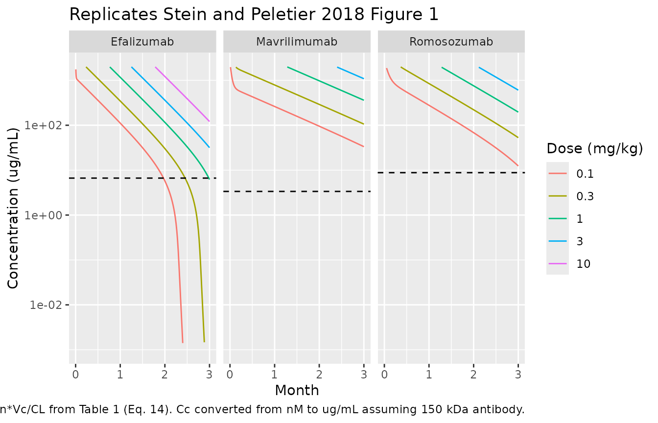
The simulated curves reproduce the visual feature highlighted in
Stein and Peletier 2018 Figure 1: as the concentration falls below
Ccrit, the slope on a log scale becomes substantially
steeper, signaling the transition from approximately-linear nonspecific
clearance to nonlinear target-mediated elimination. For romosozumab and
efalizumab the ke(R) and ke(CR) parameters are
practically unidentifiable (Stein and Peletier 2018 page 672); the
simulated curves below Ccrit therefore inherit the
very-fast complex internalization implied by Table 1
(ke(CR) = 4400/day and 860/day, respectively) and drop
steeply, exactly as in the published figure.
PKNCA validation
Because Stein and Peletier 2018 do not report numerical NCA parameters in the article text, the PKNCA pass below is a sanity check rather than a published-vs-simulated comparison. The expectations are:
- At the highest single-IV dose (10 mg/kg = 467 nmol), the initial
concentration
C0 = D / Vc(no absorption, no IIV). For mavrilimumab this is467 / 2.8 = 166.79 nM, matching the simulatedCcatt = 0. - Above
Ccritthe elimination is approximately linear with rateCL/Vc; the AUC contribution from the linear phase is approximatelyD / CLper Stein and Peletier 2018 Eq. 14 derivation.
sim_nca <- sim_all |>
  dplyr::filter(!is.na(Cc), Cc > 0) |>
  dplyr::transmute(id = paste(drug, dose_mg_per_kg, sep = "_"),
                   time = time, conc = Cc,
                   drug = drug,
                   dose_mg_per_kg = dose_mg_per_kg)
dose_df <- dplyr::bind_rows(events_mav, events_efa, events_rom) |>
  dplyr::filter(evid == 1) |>
  dplyr::transmute(id = paste(drug, dose_mg_per_kg, sep = "_"),
                   time = time, amt = amt,
                   drug = drug,
                   dose_mg_per_kg = dose_mg_per_kg)
conc_obj <- PKNCA::PKNCAconc(sim_nca, conc ~ time | drug + dose_mg_per_kg + id)
dose_obj <- PKNCA::PKNCAdose(dose_df, amt ~ time | drug + dose_mg_per_kg + id)
intervals <- data.frame(
  start = 0, end = Inf,
  cmax = TRUE, tmax = TRUE,
  aucinf.obs = TRUE, half.life = TRUE
)
nca <- PKNCA::pk.nca(PKNCA::PKNCAdata(conc_obj, dose_obj, intervals = intervals))
knitr::kable(summary(nca),
caption = "Simulated NCA parameters per drug and per single-IV dose level (typical-value, no IIV). Concentrations in nM; AUC in nM*day; half-life in day.")| start | end | drug | dose_mg_per_kg | N | cmax | tmax | half.life | aucinf.obs |
|---|---|---|---|---|---|---|---|---|
| 0 | Inf | Efalizumab | 0.1 | 1 | 19400 | 0.000 | 0.588 | 98400 |
| 0 | Inf | Efalizumab | 0.3 | 1 | 58300 | 0.000 | 0.439 | 301000 |
| 0 | Inf | Efalizumab | 1.0 | 1 | 194000 | 0.000 | 4.67 | 1.01e6 |
| 0 | Inf | Efalizumab | 3.0 | 1 | 583000 | 0.000 | 7.90 | 3.04e6 |
| 0 | Inf | Efalizumab | 10.0 | 1 | 1.94e6 | 0.000 | 9.14 | 1.01e7 |
| 0 | Inf | Mavrilimumab | 0.1 | 1 | 16700 | 0.000 | 20.4 | 153000 |
| 0 | Inf | Mavrilimumab | 0.3 | 1 | 50000 | 0.000 | 20.7 | 465000 |
| 0 | Inf | Mavrilimumab | 1.0 | 1 | 167000 | 0.000 | 20.9 | 1.55e6 |
| 0 | Inf | Mavrilimumab | 3.0 | 1 | 500000 | 0.000 | 20.9 | 4.66e6 |
| 0 | Inf | Mavrilimumab | 10.0 | 1 | 1.67e6 | 0.000 | 20.9 | 1.56e7 |
| 0 | Inf | Romosozumab | 0.1 | 1 | 19400 | 0.000 | 10.2 | 181000 |
| 0 | Inf | Romosozumab | 0.3 | 1 | 58300 | 0.000 | 14.2 | 554000 |
| 0 | Inf | Romosozumab | 1.0 | 1 | 194000 | 0.000 | 15.6 | 1.86e6 |
| 0 | Inf | Romosozumab | 3.0 | 1 | 583000 | 0.000 | 15.7 | 5.59e6 |
| 0 | Inf | Romosozumab | 10.0 | 1 | 1.94e6 | 0.000 | 15.7 | 1.87e7 |
Assumptions and deviations
-
Three model files share one vignette. Following the
replicate-author-structure default, mavrilimumab, efalizumab, and
romosozumab are packaged as three independent
Stein_2018_<drug>files because they share a structural model but have different Table 1 parameter values. The vignette covers all three because they were fit together as illustrations of one analytical result (Stein and Peletier 2018 Eq. 14). -
No IIV, no residual error. Stein and Peletier 2018
do not report between-subject variability or residual-error magnitudes
for the Table 1 fits. The packaged models are typical-value only;
rxode2::zeroRe()is unnecessary because there are no random effects to zero. -
Practical unidentifiability of
ke(R)andke(CR). Stein and Peletier 2018 page 672 (Model fit) explicitly state that the largeke(R)/ke(CR)values used for efalizumab (4400/day) and romosozumab (860/day) reflect the practical unidentifiability of these parameters from PK data. They are carried verbatim from Table 1 and should be interpreted as fitting placeholders rather than physiological rates. -
ke(R) = ke(CR)assumption. Stein and Peletier 2018 fixke(R) = ke(CR)in all three fits (Methods, Model analysis, fitting, and simulation). The packaged models reflect this assumption –lkdegandlkintare set to the same Table 1 value, but are kept as two parameters so the assumption is visible to a downstream user who wants to relax it. -
Molecular weight assumption for unit conversion.
Stein and Peletier 2018 use a 150 kDa molecular weight to convert 10
mg/kg in a 70 kg patient to 4667 nmol (page 672). The vignette uses the
same 150 kDa assumption to convert simulated
Cc(nM) toug/mLfor the Figure 1 visual comparison. -
Two-compartment QSS TMDD as a simulation tool. The
article’s primary contribution is the analytical derivation of
Ccrit, not the popPK fit per se. The Table 1 parameters are reported as illustrative typical-value fits; downstream users wanting a popPK-grade model with IIV / residual error should consult the original Bauer 1999 / Burmester 2011 / Padhi 2011 sources. - Supplementary material not consulted. Stein and Peletier 2018 reference a Supplementary Material containing the model fits to the Figure 1 data; that supplement was not available on disk during this extraction. Table 1 in the main article carries the parameter values used here, and Stein and Peletier 2018 page 672 confirms those are the values used for all simulations in the main text.