Nifedipine + captopril cardiovascular PK-PD in spontaneously hypertensive rats (Kiriyama 2024)
Source:vignettes/articles/Kiriyama_2024_nifedipine_captopril_rat.Rmd
Kiriyama_2024_nifedipine_captopril_rat.RmdModel and source
This paper contributes two model files, one per drug, because Kiriyama and colleagues fitted nifedipine and captopril independently (each drug’s PK from its own monotherapy arm, each drug’s PD from its own monotherapy arm) and then predicted the coadministration response by superposing the two separately fitted effect models. Reproducing that structure keeps the paper’s central claim – that the observed combination response differs from the additive prediction – testable.
- Nifedipine: Preclinical (rat). Two-compartment IV-infusion PK of nifedipine in spontaneously hypertensive rats (SHR/Izm) linked to four effect-compartment pharmacodynamic endpoints: mean blood pressure (BP) via a hypotensive Emax arm plus a homeostatic endogenous-hypertensive-substance (EHS) counter-regulatory arm, and heart rate (HR), QT interval (QT) and RR-corrected QT (QTc) via ordinary sigmoid Emax models. Each endpoint carries its own effect-compartment equilibration rate ke0. The BP model’s hypotensive and hypertensive arms are parameterised with Emax as the ASYMPTOTIC BP LEVEL rather than as a change from baseline (see the ini() notes). Fit by naive pooling to mean profiles in WinNonlin; the paper reports no IIV and no residual error.
- Captopril: Preclinical (rat). Two-compartment IV-infusion PK of captopril in spontaneously hypertensive rats (SHR/Izm) linked to three effect-compartment pharmacodynamic endpoints – mean blood pressure (BP), heart rate (HR) and QT interval (QT) – each an ordinary sigmoid Emax model with its own effect-compartment equilibration rate ke0. Unlike its nifedipine sister model, captopril’s BP response needed no homeostatic counter-regulation arm; the HR and QT ke0 values are so small (1e-5 /min) that those two effect compartments behave as cumulative-exposure integrators. Fit by naive pooling to mean profiles in WinNonlin; the paper reports no IIV and no residual error.
- Citation: Kiriyama A, Kimura S, Yamashita S. Exploring the multiple effects of nifedipine and captopril administration in spontaneously hypertensive rats through pharmacokinetic-pharmacodynamic analyses. Pharmacol Res Perspect. 2024;12(4):e1249. doi:10.1002/prp2.1249. Sister model file from the same paper: modellib(‘Kiriyama_2024_captopril_rat’). The BP homeostasis (EHS feedback) structure was first reported by the same group in Kiriyama A et al. (reference 5 of the 2024 paper), a nifedipine + propranolol SHR study; the 2024 paper restates the full equation set, so no upstream source is required.
- Article: https://doi.org/10.1002/prp2.1249
nif <- rxode2::rxode2(readModelDb("Kiriyama_2024_nifedipine_rat"))
cap <- rxode2::rxode2(readModelDb("Kiriyama_2024_captopril_rat"))
Population
Male spontaneously hypertensive rats (SHR/Izm, 215-315 g) were anaesthetised with intraperitoneal urethane (1.0 g/kg), catheterised in the left carotid artery for blood pressure and instrumented for ECG. Blood pressure (BP), heart rate (HR) and QT interval were recorded continuously from -15 to 180 min after the start of a 30-minute intravenous infusion into the right femoral vein; plasma was sampled from the right jugular vein between 5 and 300 min and assayed by LC-MS/MS (Methods sections 2.2-2.3).
Monotherapy doses were nifedipine 1.0 mg/kg and captopril 15.0 mg/kg. For coadministration both doses were reduced – nifedipine 0.5 mg/kg and captopril 5.0 mg/kg – chosen so that the combination would produce an effect comparable to either drug alone. Group sizes differ by analysis: the PK parameters of Tables 1 and 2 come from 3-6 rats, the PD parameters of Table 3 from 8-10 rats. The paper reports that baseline BP, HR and QT did not differ significantly across the nifedipine, captopril and coadministration groups.
The same information is available programmatically via each model’s
population metadata
(readModelDb("Kiriyama_2024_nifedipine_rat")()$population).
Dose scale: recovering the body weight
The paper reports doses in mg/kg but fits absolute
central volumes (mL) and absolute micro-constants, so converting a dose
to an event-table amt requires a body weight that the paper
never states beyond the 215-315 g range. It is recoverable: the Table 2
parameters plus the Figure 2 fitted peak concentrations pin it down, and
the two drugs give independent estimates.
# Peak of the fitted (solid) monotherapy curves read from Figure 2.
fig2_peak <- c(nifedipine = 2900, captopril = 19500)

peak_per_mg <- function(mod, pars) {
  ev <- rbind(
    data.frame(time = 0, amt = 1e6, dur = 30, evid = 1L,
               cmt = "central", dvid = NA_integer_),
    data.frame(time = seq(0, 60, by = 1), amt = NA_real_, dur = NA_real_,
               evid = 0L, cmt = "central", dvid = 1L)
  )
  s <- rxode2::rxSolve(mod, ev, params = pars, returnType = "data.frame",
                       useLinCmt = FALSE, atol = 1e-12, rtol = 1e-12)
  s$Cc[s$time == 30]   # ng/mL per 1 mg infused over 30 min
}

nif_pk_mono <- c(lvc = log(54.9), lkel = log(0.0218), lk12 = log(0.0121), lk21 = log(0.0165))
cap_pk_mono <- c(lvc = log(54.2), lkel = log(0.0521), lk12 = log(0.1530), lk21 = log(0.0694))

implied_g <- c(
  nifedipine = 1000 * (fig2_peak[["nifedipine"]] / peak_per_mg(nif, nif_pk_mono)) / 1.0,
  captopril  = 1000 * (fig2_peak[["captopril"]]  / peak_per_mg(cap, cap_pk_mono)) / 15.0
)
round(implied_g, 1)
#> nifedipine  captopril
#>      247.2      248.8
Both drugs independently imply a rat of about 250 g – agreeing to within 1% of each other and comfortably inside the reported 215-315 g range. Every simulation below therefore doses a 250 g rat.
Source trace
Every ini() entry in both model files carries an in-file
comment naming its source location. They are collected here for
review.
| Model | Equation / parameter | Value | Source location |
|---|---|---|---|
| both |
d/dt(central), d/dt(peripheral1)
(2-compartment, zero-order infusion) |
n/a | Methods 2.4 equations; Figure 1 |
| both |
d/dt(effect_*) = ke0 * (Cc - effect)
|
n/a | Methods 2.5, dC3/dt equation |
| both |
hr, qt, qtc sigmoid Emax |
n/a | Methods 2.5,
E = E0 -/+ Emax*C3^gamma/(EC50^gamma + C3^gamma); Figure
1B |
| nifedipine |
bp (hypotensive + EHS hypertensive arms) |
n/a | Methods 2.5 dE/dt equation; Figure 1A |
| nifedipine | d/dt(ehs) |
n/a | Methods 2.5 dC4/dt equation (see Errata) |
| nifedipine |
lvc / lkel / lk12 /
lk21
|
54.9 mL / 0.0218 / 0.0121 / 0.0165 min-1 | Table 2, nifedipine Monotherapy |
| nifedipine |
lke0_bp, le0_bp, lemax_bp,
lec50_bp
|
0.135 min-1, 96.8, 67.1 mmHg, 86.3 ng/mL | Table 3, nifedipine BP |
| nifedipine |
lkin_ehs, lkout_ehs,
lgamma_bp
|
0.0217 unit/min, 0.0119 min-1, 1.17 | Table 3, nifedipine BP (KEHS,in, kEHS,out, alpha) |
| nifedipine |
lemax_bp_ehs, lec50_bp_ehs
|
49 338 mmHg, 1450 unit | Table 3, nifedipine BP (Emax,2, EC50,2) |
| nifedipine |
lke0_hr, le0_hr, lemax_hr,
lec50_hr, lhill_hr
|
0.006589 min-1, 306, 63.3 beat/min, 115 ng/mL, 0.931 | Table 3, nifedipine HR |
| nifedipine |
lke0_qt, le0_qt, lemax_qt,
lec50_qt, lhill_qt
|
0.0117 min-1, 75.8, 76.3 msec, 3227 ng/mL, 0.857 | Table 3, nifedipine QT |
| nifedipine |
lke0_qtc, le0_qtc, lemax_qtc,
lec50_qtc, lhill_qtc
|
0.0130 min-1, 169, 29.5 msec, 522 ng/mL, 1.92 | Results prose (Figure 3D paragraph), not Table 3 |
| captopril |
lvc / lkel / lk12 /
lk21
|
54.2 mL / 0.0521 / 0.153 / 0.0694 min-1 | Table 2, captopril Monotherapy |
| captopril |
lke0_bp, le0_bp, lemax_bp,
lec50_bp, lhill_bp
|
0.0400 min-1, 105, 41.8 mmHg, 7885 ng/mL, 0.662 | Table 3, captopril BP |
| captopril |
lke0_hr, le0_hr, lemax_hr,
lec50_hr, lhill_hr
|
1.21e-5 min-1, 312.8, 80.4 beat/min, 7.6 ng/mL, 1.4 | Table 3, captopril HR |
| captopril |
lke0_qt, le0_qt, lemax_qt,
lec50_qt, lhill_qt
|
4.05e-5 min-1, 81.2, 41.9 msec, 4873 ng/mL, 0.1347 | Table 3, captopril QT |
| both | coadministration PK override
(lvc/lkel/lk12/lk21) |
nifedipine 26.7 mL, 0.0768, 0.132, 0.0764; captopril 41.7 mL, 0.0842, 0.0631, 0.0529 | Table 2, Combination columns |
| both | residual error and IIV | not reported (fixed(0), no etas) |
Methods 2.4-2.5 (WinNonlin fits to mean profiles; only AIC reported) |
Virtual cohort
The models are deterministic: the paper fitted mean profiles by naive
pooling in WinNonlin and reported no inter-individual variability and no
residual error, so neither model file carries eta terms.
Each arm is therefore a single typical 250 g rat rather than a sampled
cohort, and no zeroRe() / omega = NA step is
needed (there is nothing to zero). This is far below the 200-per-arm
cap.
# Table 2 parameter sets. The paper reports a separate PK fit for each drug under
# monotherapy and under coadministration; it applies them by scenario rather than
# as a covariate effect, because it concludes that none of the PK differences
# reached statistical significance.
pk_sets <- list(
  nif_mono  = nif_pk_mono,
  nif_combo = c(lvc = log(26.7), lkel = log(0.0768), lk12 = log(0.132),  lk21 = log(0.0764)),
  cap_mono  = cap_pk_mono,
  cap_combo = c(lvc = log(41.7), lkel = log(0.0842), lk12 = log(0.0631), lk21 = log(0.0529))
)

# One arm = one solve, because rxSolve applies `params` globally and each arm
# needs a different PK parameter set. `id` and `arm` are assigned explicitly
# rather than via `keep`, since rxSolve drops `id` for a single-subject solve.
run_arm <- function(mod, pars, mg_per_kg, arm, id, tmax = 300, by = 1) {
  ev <- rbind(
    data.frame(time = 0, amt = mg_per_kg * WT * 1e6, dur = 30, evid = 1L,
               cmt = "central", dvid = NA_integer_),
    data.frame(time = seq(0, tmax, by = by), amt = NA_real_, dur = NA_real_,
               evid = 0L, cmt = "central", dvid = 1L)
  )
  out <- rxode2::rxSolve(mod, ev, params = pars, returnType = "data.frame",
                         useLinCmt = FALSE, atol = 1e-12, rtol = 1e-12)
  out$id <- id
  out$arm <- arm
  out$mg_per_kg <- mg_per_kg
  out$amt_ng <- mg_per_kg * WT * 1e6
  out
}
Simulation
sims <- dplyr::bind_rows(
  # Figure 2 solid curves: monotherapy fits.
  run_arm(nif, pk_sets$nif_mono,  1.0, "Nifedipine 1.0 mg/kg (mono)",   1L),
  run_arm(cap, pk_sets$cap_mono, 15.0, "Captopril 15 mg/kg (mono)",     2L),
  # Figure 2 bold-solid curves: coadministration fits.
  run_arm(nif, pk_sets$nif_combo, 0.5, "Nifedipine 0.5 mg/kg (combo)",  3L),
  run_arm(cap, pk_sets$cap_combo, 5.0, "Captopril 5.0 mg/kg (combo)",   4L),
  # Figure 2 dashed curves: reduced dose predicted from the MONOTHERAPY PK.
  run_arm(nif, pk_sets$nif_mono,  0.5, "Nifedipine 0.5 mg/kg (predicted from mono PK)", 5L),
  run_arm(cap, pk_sets$cap_mono,  5.0, "Captopril 5.0 mg/kg (predicted from mono PK)",  6L)
)

drug_of <- function(a) ifelse(grepl("^Nifedipine", a), "Nifedipine", "Captopril")
sims$drug <- drug_of(sims$arm)
Dose linearity
The paper states the PK “were nearly linear within these dosage ranges”, which is what licenses reusing the monotherapy PD parameters for the reduced coadministration doses. With a fixed parameter set the model is exactly linear in dose, so halving the nifedipine dose must halve every concentration. This is a free, exact check on the infusion encoding.
lin <- sims |>
  dplyr::filter(arm %in% c("Nifedipine 1.0 mg/kg (mono)",
                           "Nifedipine 0.5 mg/kg (predicted from mono PK)"),
                time > 0) |>
  dplyr::select(time, arm, Cc) |>
  tidyr::pivot_wider(names_from = arm, values_from = Cc)

ratio <- lin[["Nifedipine 0.5 mg/kg (predicted from mono PK)"]] /
  lin[["Nifedipine 1.0 mg/kg (mono)"]]
stopifnot(max(abs(ratio - 0.5)) < 1e-8)
range(ratio)
#> [1] 0.5 0.5
Replicate published figures
Figure 2 – plasma concentrations
# Replicates Figure 2 of Kiriyama 2024: fitted plasma nifedipine (A) and
# captopril (B) after a 30-min IV infusion, monotherapy vs coadministration,
# plus the reduced dose predicted from the monotherapy PK (dashed in the paper).
sims |>
  ggplot(aes(time, Cc, colour = arm, linetype = arm)) +
  geom_line(linewidth = 0.7) +
  facet_wrap(~drug, scales = "free_y") +
  scale_x_continuous(breaks = seq(0, 300, by = 60)) +
  guides(colour = guide_legend(ncol = 1), linetype = guide_legend(ncol = 1)) +
  theme(legend.position = "bottom", legend.title = ggplot2::element_blank()) +
  labs(x = "Time (min)", y = "Plasma concentration (ng/mL)",
       title = "Figure 2 - fitted plasma concentrations",
       caption = "Replicates Figure 2 of Kiriyama 2024.")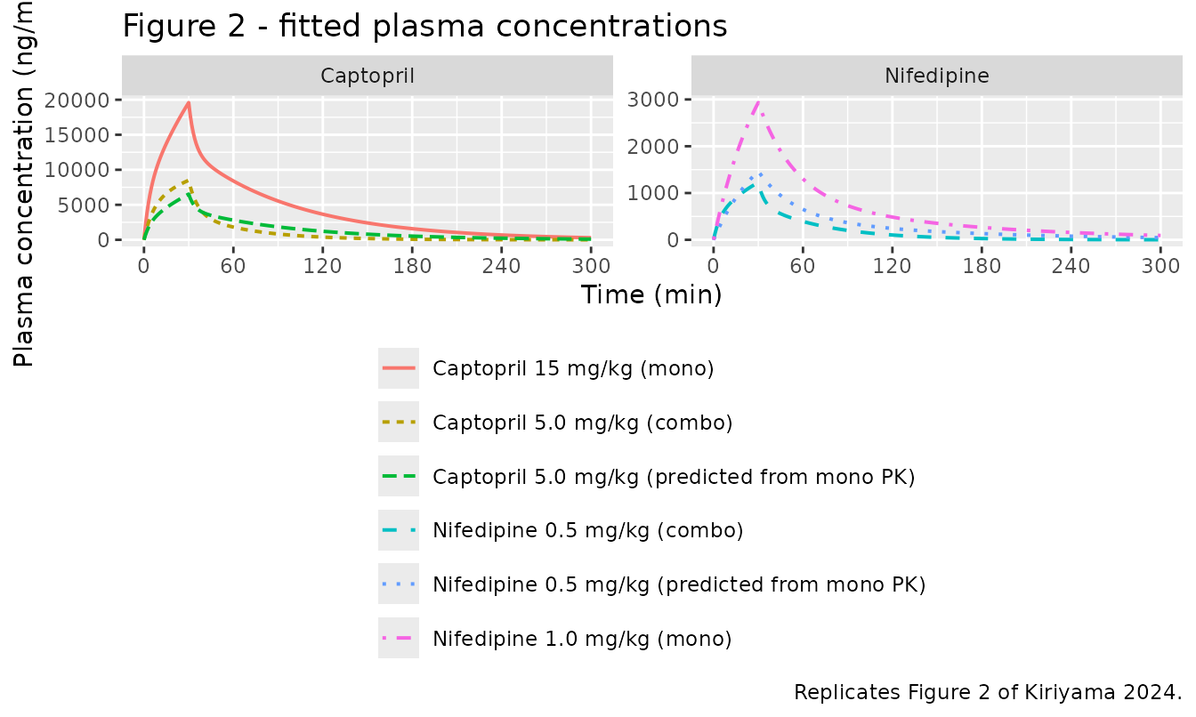
peak30 <- sims |>
  dplyr::filter(time == 30) |>
  dplyr::select(arm, Cc) |>
  dplyr::mutate(Cc = round(Cc))
knitr::kable(
  peak30 |> dplyr::rename("Arm" = arm, "Cc at 30 min (ng/mL)" = Cc),
  caption = "End-of-infusion concentrations. Figure 2 read-offs: 2900 and 19500 ng/mL for the monotherapy solid curves, ~1200 and ~8300 ng/mL for the coadministration bold-solid curves."
)| Arm | Cc at 30 min (ng/mL) |
|---|---|
| Nifedipine 1.0 mg/kg (mono) | 2933 |
| Captopril 15 mg/kg (mono) | 19591 |
| Nifedipine 0.5 mg/kg (combo) | 1227 |
| Captopril 5.0 mg/kg (combo) | 8492 |
| Nifedipine 0.5 mg/kg (predicted from mono PK) | 1466 |
| Captopril 5.0 mg/kg (predicted from mono PK) | 6530 |
Figure 3 – pharmacodynamics during monotherapy
# Replicates Figure 3 of Kiriyama 2024: BP (A), HR (B), QT (C) and QTc (D)
# after nifedipine 1.0 mg/kg or captopril 15 mg/kg. QTc was only quantifiable
# for nifedipine (see Errata).
pd_long <- sims |>
  dplyr::filter(arm %in% c("Nifedipine 1.0 mg/kg (mono)", "Captopril 15 mg/kg (mono)"),
                time <= 180) |>
  dplyr::select(time, drug, bp, hr, qt, dplyr::any_of("qtc")) |>
  tidyr::pivot_longer(c(bp, hr, qt, dplyr::any_of("qtc")),
                      names_to = "endpoint", values_to = "value") |>
  dplyr::filter(!is.na(value)) |>
  dplyr::mutate(endpoint = factor(
    endpoint, levels = c("bp", "hr", "qt", "qtc"),
    labels = c("A: BP (mmHg)", "B: HR (beat/min)",
               "C: QT (msec)", "D: QTc (msec)")
  ))

pd_long |>
  ggplot(aes(time, value, colour = drug)) +
  geom_line(linewidth = 0.7) +
  facet_wrap(~endpoint, scales = "free_y") +
  scale_x_continuous(breaks = seq(0, 180, by = 60)) +
  theme(legend.position = "bottom", legend.title = ggplot2::element_blank()) +
  labs(x = "Time (min)", y = NULL,
       title = "Figure 3 - PD responses during monotherapy",
       caption = "Replicates Figure 3 of Kiriyama 2024. QTc (panel D) is nifedipine only.")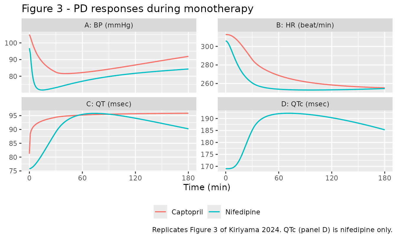
Gates against the paper’s own reported PD values
mono <- sims |> dplyr::filter(time <= 180)
nifm <- mono |> dplyr::filter(arm == "Nifedipine 1.0 mg/kg (mono)")
capm <- mono |> dplyr::filter(arm == "Captopril 15 mg/kg (mono)")

pd_checks <- tibble::tibble(
  Quantity = c("Nifedipine BP nadir (mmHg)",
               "Nifedipine BP nadir time (min)",
               "Nifedipine BP at 180 min (mmHg)",
               "Nifedipine HR at 180 min (beat/min)",
               "Captopril BP nadir (mmHg)",
               "Captopril HR at 180 min (beat/min)",
               "Captopril QT at 180 min (msec)"),
  Simulated = c(round(min(nifm$bp), 1),
                nifm$time[which.min(nifm$bp)],
                round(nifm$bp[nifm$time == 180], 1),
                round(nifm$hr[nifm$time == 180], 1),
                round(min(capm$bp), 1),
                round(capm$hr[capm$time == 180], 1),
                round(capm$qt[capm$time == 180], 1)),
  Paper = c("70.9 +/- 8.6 (measured Emax, Results)",
            "~10 (Results: 'approximately 10 min')",
            "~85-88 (Figure 3A)",
            "~250 (Results: 'approximately 250 beats/min')",
            "~80 at 40-60 min (Figure 3A)",
            "~250 (Results)",
            "~95-98 (Figure 3C)")
)
knitr::kable(pd_checks, caption = "Simulated PD landmarks against the values Kiriyama 2024 reports in its Results text and draws in Figure 3.")| Quantity | Simulated | Paper |
|---|---|---|
| Nifedipine BP nadir (mmHg) | 71.7 | 70.9 +/- 8.6 (measured Emax, Results) |
| Nifedipine BP nadir time (min) | 15.0 | ~10 (Results: ‘approximately 10 min’) |
| Nifedipine BP at 180 min (mmHg) | 84.3 | ~85-88 (Figure 3A) |
| Nifedipine HR at 180 min (beat/min) | 254.6 | ~250 (Results: ‘approximately 250 beats/min’) |
| Captopril BP nadir (mmHg) | 81.6 | ~80 at 40-60 min (Figure 3A) |
| Captopril HR at 180 min (beat/min) | 255.3 | ~250 (Results) |
| Captopril QT at 180 min (msec) | 95.9 | ~95-98 (Figure 3C) |
stopifnot(
  # Nifedipine BP nadir sits inside the paper's measured Emax 70.9 +/- 8.6 mmHg,
  # and is pinned exactly as a regression guard.
  abs(min(nifm$bp) - 71.7) < 0.05,
  min(nifm$bp) > 70.9 - 8.6, min(nifm$bp) < 70.9 + 8.6,
  nifm$time[which.min(nifm$bp)] == 15,
  # BP recovers but never back to the 96.8 mmHg baseline (Figure 3A).
  nifm$bp[nifm$time == 180] > 80, nifm$bp[nifm$time == 180] < 90,
  max(nifm$bp) <= 96.8 + 1e-8,
  # The hypotensive arm's asymptote is a BP LEVEL of 67.1 mmHg, so BP can never
  # fall below it. Reading Emax,1 as a 67.1 mmHg decrease would allow ~29.7 mmHg.
  min(nifm$bp) > 67.1,
  # Both drugs converge on ~250 beat/min after 60-90 min (Results).
  abs(nifm$hr[nifm$time == 180] - 250) < 10,
  abs(capm$hr[capm$time == 180] - 250) < 10,
  # Captopril HR cannot fall below its own floor E0 - Emax = 232.4 beat/min.
  min(capm$hr) > 312.8 - 80.4,
  # Captopril QT plateau (Figure 3C).
  abs(capm$qt[capm$time == 180] - 96.5) < 2
)
Drug-free gate on the BP homeostasis model
The nifedipine BP model is the only structure in the paper that
required reinterpretation (see Errata). The decisive check is that with
no drug at all the model must hold BP exactly at its
baseline E0, which is precisely what the paper’s stated
initial condition (C3 = 0, C4 = 0,
E = E0) asserts. This is a runtime gate rather than a
comment because it is the single assertion that distinguishes the
correct reading of the EHS production term from the incorrect one.
ev0 <- rbind(
  data.frame(time = 0, amt = 0, dur = 30, evid = 1L, cmt = "central", dvid = NA_integer_),
  data.frame(time = seq(0, 180, by = 1), amt = NA_real_, dur = NA_real_,
             evid = 0L, cmt = "central", dvid = 1L)
)
s0 <- rxode2::rxSolve(nif, ev0, params = pk_sets$nif_mono, returnType = "data.frame",
                      useLinCmt = FALSE, atol = 1e-12, rtol = 1e-12)

c(max_bp_deviation_mmHg = max(abs(s0$bp - 96.8)), max_ehs = max(abs(s0$ehs)))
#> max_bp_deviation_mmHg               max_ehs
#>          2.842171e-14          3.013225e-16
stopifnot(max(abs(s0$bp - 96.8)) < 1e-6, max(abs(s0$ehs)) < 1e-6)
Figure 4 – pharmacodynamics during coadministration
The paper predicts the combination response by superposing each drug’s separately fitted effect (Methods 2.6):
- BP and HR:
Emix = E0 - ((E0 - E_nifedipine) + (E0 - E_captopril)) - QT:
Emix = E0 + ((E_nifedipine - E0) + (E_captopril - E0))
Both forms reduce to summing each drug’s deviation from its own baseline and adding it back onto a common baseline. Because the two model files carry different fitted baselines for the same endpoint (BP: 96.8 vs 105 mmHg), the common baseline has to be chosen; the nifedipine baseline is used here and the choice is recorded in the Errata.
# Replicates Figure 4 of Kiriyama 2024: BP (A), HR (B) and QT (C) during
# coadministration of nifedipine 0.5 mg/kg and captopril 5.0 mg/kg, using the
# coadministration PK of Table 2 and the monotherapy PD of Table 3, together
# with the paper's additive prediction (bold solid line in the paper).
nifc <- sims |> dplyr::filter(arm == "Nifedipine 0.5 mg/kg (combo)", time <= 180)
capc <- sims |> dplyr::filter(arm == "Captopril 5.0 mg/kg (combo)",  time <= 180)

e0_nif <- c(bp = 96.8, hr = 306,   qt = 75.8)
e0_cap <- c(bp = 105,  hr = 312.8, qt = 81.2)

additive <- tibble::tibble(
  time = nifc$time,
  bp = (nifc$bp - e0_nif[["bp"]]) + (capc$bp - e0_cap[["bp"]]) + e0_nif[["bp"]],
  hr = (nifc$hr - e0_nif[["hr"]]) + (capc$hr - e0_cap[["hr"]]) + e0_nif[["hr"]],
  qt = (nifc$qt - e0_nif[["qt"]]) + (capc$qt - e0_cap[["qt"]]) + e0_nif[["qt"]]
)

combo_long <- dplyr::bind_rows(
  nifc     |> dplyr::select(time, bp, hr, qt) |> dplyr::mutate(series = "Nifedipine 0.5 mg/kg"),
  capc     |> dplyr::select(time, bp, hr, qt) |> dplyr::mutate(series = "Captopril 5.0 mg/kg"),
  additive |> dplyr::mutate(series = "Additive prediction")
) |>
  tidyr::pivot_longer(c(bp, hr, qt), names_to = "endpoint", values_to = "value") |>
  dplyr::mutate(endpoint = factor(endpoint, levels = c("bp", "hr", "qt"),
                                  labels = c("A: BP (mmHg)", "B: HR (beat/min)",
                                             "C: QT (msec)")))

combo_long |>
  ggplot(aes(time, value, colour = series, linewidth = series)) +
  geom_line() +
  facet_wrap(~endpoint, scales = "free_y") +
  scale_linewidth_manual(values = c("Additive prediction" = 1.1,
                                    "Nifedipine 0.5 mg/kg" = 0.6,
                                    "Captopril 5.0 mg/kg" = 0.6)) +
  scale_x_continuous(breaks = seq(0, 180, by = 60)) +
  theme(legend.position = "bottom", legend.title = ggplot2::element_blank()) +
  labs(x = "Time (min)", y = NULL,
       title = "Figure 4 - PD responses during coadministration",
       caption = "Replicates Figure 4 of Kiriyama 2024; the bold line is the paper's additive prediction.")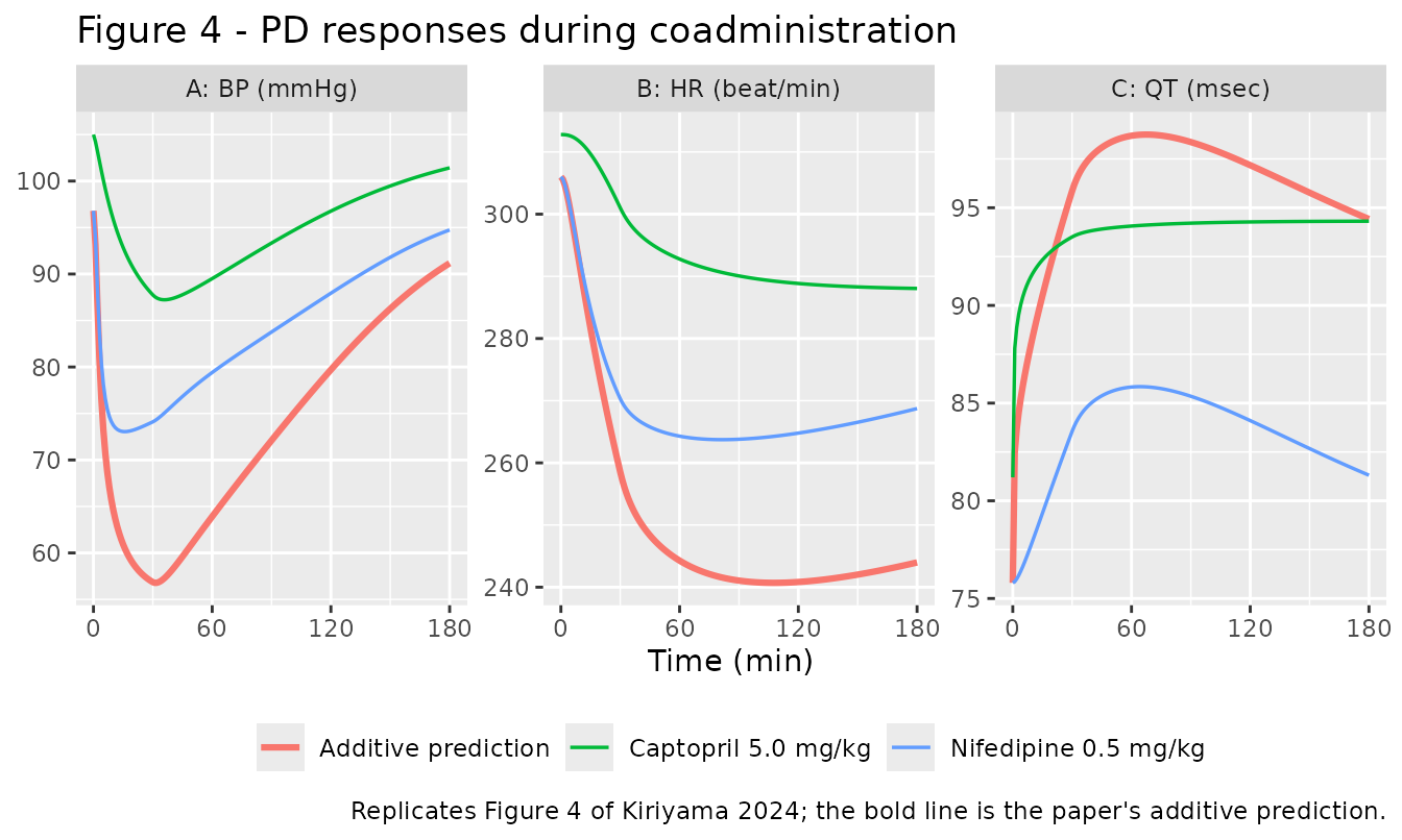
The paper’s qualitative conclusions about the combination are reproduced: the early BP fall is dominated by nifedipine, captopril contributes little to HR at 5.0 mg/kg, and the additive prediction sits below each single agent for QT.
combo_checks <- tibble::tibble(
  Quantity = c("BP nadir, nifedipine arm (mmHg)",
               "BP nadir, additive prediction (mmHg)",
               "HR change from baseline, captopril arm at 180 min (beat/min)",
               "QT at 180 min, additive prediction (msec)"),
  Simulated = c(round(min(nifc$bp), 1), round(min(additive$bp), 1),
                round(capc$hr[capc$time == 180] - e0_cap[["hr"]], 1),
                round(additive$qt[additive$time == 180], 1))
)
knitr::kable(combo_checks, caption = "Coadministration landmarks. The paper reports a measured combination BP Emax of 75.0 +/- 4.8 mmHg approximately 10 min after infusion start (Results, Figure 4A).")| Quantity | Simulated |
|---|---|
| BP nadir, nifedipine arm (mmHg) | 73.0 |
| BP nadir, additive prediction (mmHg) | 56.8 |
| HR change from baseline, captopril arm at 180 min (beat/min) | -24.8 |
| QT at 180 min, additive prediction (msec) | 94.4 |
stopifnot(
  # The paper: "the alteration in BP during coadministration was nearly equal to
  # that produced by nifedipine", with measured Emax 75.0 +/- 4.8 mmHg.
  min(nifc$bp) > 75.0 - 4.8, min(nifc$bp) < 75.0 + 4.8,
  # Captopril's own HR contribution at 5.0 mg/kg is modest ("Captopril exhibited
  # minimal effects on HR at this dose") but not zero.
  capc$hr[capc$time == 180] - e0_cap[["hr"]] < 0,
  # The additive prediction must be more extreme than either single agent for BP.
  min(additive$bp) < min(nifc$bp)
)
PKNCA validation
Table 1 of the paper reports moment-analysis NCA for all four dose arms. The NCA below runs on the model-predicted profiles over the paper’s own 5-300 min sampling window, using the PK parameter set matching each arm.
nca_arms <- c("Nifedipine 1.0 mg/kg (mono)", "Nifedipine 0.5 mg/kg (combo)",
              "Captopril 15 mg/kg (mono)",   "Captopril 5.0 mg/kg (combo)")

sim_nca <- sims |>
  dplyr::filter(arm %in% nca_arms, !is.na(Cc)) |>
  dplyr::select(id, time, Cc, arm)

# Guarantee a time = 0 row per arm; for a 30-min infusion the pre-dose
# concentration is 0.
sim_nca <- dplyr::bind_rows(
  sim_nca,
  sim_nca |> dplyr::distinct(id, arm) |> dplyr::mutate(time = 0, Cc = 0)
) |>
  dplyr::distinct(id, arm, time, .keep_all = TRUE) |>
  dplyr::arrange(id, arm, time)

dose_df <- sims |>
  dplyr::filter(arm %in% nca_arms) |>
  dplyr::distinct(id, arm, amt_ng) |>
  dplyr::mutate(time = 0, amt = amt_ng, dur = 30) |>
  dplyr::select(id, time, amt, dur, arm)

conc_obj <- PKNCA::PKNCAconc(sim_nca, Cc ~ time | arm + id,
                             concu = "ng/mL", timeu = "min")
# `duration` is mandatory for an infusion: without it PKNCA treats the dose as a
# bolus and the IV MRT / Vss are inflated by dur/2.
dose_obj <- PKNCA::PKNCAdose(dose_df, amt ~ time | arm + id,
                             route = "intravascular", duration = "dur",
                             doseu = "ng")

intervals <- data.frame(
  start = 0, end = Inf,
  cmax = TRUE, tmax = TRUE, aucinf.obs = TRUE, half.life = TRUE,
  cl.obs = TRUE, vz.obs = TRUE, mrt.iv.obs = TRUE
)

nca_res <- PKNCA::pk.nca(PKNCA::PKNCAdata(conc_obj, dose_obj, intervals = intervals))
Comparison against published NCA (Table 1)
Two transcription notes. First, Table 1 reports AUC in ugmin/mL;
the values below are multiplied by 1000 so both sides are in
ngmin/mL. Second, the paper states that “the volume of distribution
at steady state (Vdss) was calculated using CLtot/ke” – that is CL
divided by the terminal rate constant, which is Vz, not
Vss. The Table 1 “Vdss” row is therefore compared against PKNCA’s
vz.obs.
published <- tibble::tribble(
  ~arm,                            ~aucinf.obs, ~half.life, ~cl.obs, ~vz.obs, ~mrt.iv.obs,
  "Nifedipine 1.0 mg/kg (mono)",      237e3,        69.0,     1.35,     162,        82.8,
  "Nifedipine 0.5 mg/kg (combo)",      63.4e3,      53.8,     2.24,     161,        39.0,
  "Captopril 15 mg/kg (mono)",       1730e3,        81.6,     4.21,     395,        69.8,
  "Captopril 5.0 mg/kg (combo)",      411e3,       190.0,     4.92,    1565,        98.9
)

cmp <- nlmixr2lib::ncaComparisonTable(
  simulated = nca_res,
  reference = published,
  by        = "arm",
  units     = c(aucinf.obs = "ng*min/mL", half.life = "min", cl.obs = "mL/min",
                vz.obs = "mL", mrt.iv.obs = "min"),
  tolerance_pct = 20
)

knitr::kable(cmp, caption = "Simulated vs Kiriyama 2024 Table 1. * differs from the reference by >20%.")| NCA parameter | arm | Reference | Simulated | % diff |
|---|---|---|---|---|
| AUC0-∞ (obs) (ng*min/mL) | Nifedipine 1.0 mg/kg (mono) | 237000 | 209000 | -11.9% |
| AUC0-∞ (obs) (ng*min/mL) | Nifedipine 0.5 mg/kg (combo) | 63400 | 61000 | -3.9% |
| AUC0-∞ (obs) (ng*min/mL) | Captopril 15 mg/kg (mono) | 1730000 | 1330000 | -23.2%* |
| AUC0-∞ (obs) (ng*min/mL) | Captopril 5.0 mg/kg (combo) | 411000 | 356000 | -13.4% |
| t½ (min) | Nifedipine 1.0 mg/kg (mono) | 69 | 79.1 | +14.7% |
| t½ (min) | Nifedipine 0.5 mg/kg (combo) | 53.8 | 31 | -42.4%* |
| t½ (min) | Captopril 15 mg/kg (mono) | 81.6 | 49.8 | -38.9%* |
| t½ (min) | Captopril 5.0 mg/kg (combo) | 190 | 27.1 | -85.7%* |
| CL/F (mL/min) | Nifedipine 1.0 mg/kg (mono) | 1.35 | 1.2 | -11.3% |
| CL/F (mL/min) | Nifedipine 0.5 mg/kg (combo) | 2.24 | 2.05 | -8.4% |
| CL/F (mL/min) | Captopril 15 mg/kg (mono) | 4.21 | 2.82 | -32.9%* |
| CL/F (mL/min) | Captopril 5.0 mg/kg (combo) | 4.92 | 3.51 | -28.6%* |
| MRT (IV) (min) | Nifedipine 1.0 mg/kg (mono) | 82.8 | 79.1 | -4.4% |
| MRT (IV) (min) | Nifedipine 0.5 mg/kg (combo) | 39 | 35.5 | -8.9% |
| MRT (IV) (min) | Captopril 15 mg/kg (mono) | 69.8 | 61.5 | -11.9% |
| MRT (IV) (min) | Captopril 5.0 mg/kg (combo) | 98.9 | 26.1 | -73.7%* |
| Vz/F (mL) | Nifedipine 1.0 mg/kg (mono) | 162 | 137 | -15.6% |
| Vz/F (mL) | Nifedipine 0.5 mg/kg (combo) | 161 | 91.6 | -43.1%* |
| Vz/F (mL) | Captopril 15 mg/kg (mono) | 395 | 203 | -48.6%* |
| Vz/F (mL) | Captopril 5.0 mg/kg (combo) | 1560 | 137 | -91.2%* |
attr(cmp, "footnote")
#> [1] "* differs from reference by more than ±20%."
Ten of the twenty rows are starred. The reason is methodological rather than a transcription error, but it is worth being specific about which explanation actually holds.
Table 1 is a moment analysis of individual animals, then
averaged (3-6 rats per arm, i.e. mean(D / AUC_i)),
whereas Table 2 – the parameter set these model files encode – is a
naive-pooled fit to the mean profile
(D / AUC_mean). Those two estimators diverge whenever the
between-animal spread is wide, and here it is extreme: several of Table
1’s own standard deviations equal or exceed their means
(CLtot 4.21 +/- 4.25 mL/min for captopril monotherapy,
Vdss 1565 +/- 1695 mL and t1/2 190 +/- 157 min
for captopril combination). The paper itself flags a mismatch between
its two tables – “the Cmax of nifedipine was overestimated during
monotherapy, whereas for captopril, it was underestimated”.
One candidate explanation was tested and rejected:
the paper estimates t1/2 by “linear regression of three
minimal data points from the terminal portion”. Recomputing the
simulated t1/2 that way – restricting the profile to the
Figure 2 sampling times and regressing only the last three – reproduces
PKNCA’s default almost exactly (nifedipine monotherapy 79.5 vs 79.1 min;
captopril monotherapy 50.0 vs 49.8 min), so the terminal-slope rule is
not what separates the two tables. That explanation is
therefore not offered.
The informative comparison for this paper is containment within Table 1’s own reported variability, since a 20% tolerance is far tighter than the data support:
published_sd <- tibble::tribble(
  ~arm,   ~param,        ~mean,   ~sd,
  nca_arms[1], "aucinf.obs",  237e3,   85e3,
  nca_arms[2], "aucinf.obs",   63.4e3, 23.4e3,
  nca_arms[3], "aucinf.obs", 1730e3,  411e3,
  nca_arms[4], "aucinf.obs",  411e3,  407e3,
  nca_arms[1], "half.life",    69.0,   41.9,
  nca_arms[2], "half.life",    53.8,   17.1,
  nca_arms[3], "half.life",    81.6,   58.4,
  nca_arms[4], "half.life",   190.0,  157.0,
  nca_arms[1], "cl.obs",        1.35,   0.57,
  nca_arms[2], "cl.obs",        2.24,   1.30,
  nca_arms[3], "cl.obs",        4.21,   4.25,
  nca_arms[4], "cl.obs",        4.92,   2.57,
  nca_arms[1], "vz.obs",      162,    171,
  nca_arms[2], "vz.obs",      161,     61,
  nca_arms[3], "vz.obs",      395,    334,
  nca_arms[4], "vz.obs",     1565,   1695,
  nca_arms[1], "mrt.iv.obs",   82.8,   60.8,
  nca_arms[2], "mrt.iv.obs",   39.0,    3.6,
  nca_arms[3], "mrt.iv.obs",   69.8,   26.7,
  nca_arms[4], "mrt.iv.obs",   98.9,   70.5
)

sim_vals <- as.data.frame(nca_res$result) |>
  dplyr::filter(start == 0, is.infinite(end)) |>
  dplyr::select(arm, param = PPTESTCD, simulated = PPORRES)

containment <- published_sd |>
  dplyr::left_join(sim_vals, by = c("arm", "param")) |>
  dplyr::mutate(
    Parameter = nlmixr2lib::ncaParamLabel(param),
    `Table 1 mean +/- SD` = paste0(signif(mean, 3), " +/- ", signif(sd, 3)),
    Simulated = signif(simulated, 3),
    `Within 1 SD` = ifelse(simulated >= mean - sd & simulated <= mean + sd, "yes", "NO")
  )

knitr::kable(
  containment |> dplyr::select(Parameter, arm, `Table 1 mean +/- SD`, Simulated, `Within 1 SD`) |>
    dplyr::rename("Arm" = arm),
  caption = "Simulated NCA against Table 1's own mean +/- 1 SD."
)| Parameter | Arm | Table 1 mean +/- SD | Simulated | Within 1 SD |
|---|---|---|---|---|
| AUC0-∞ (obs) | Nifedipine 1.0 mg/kg (mono) | 237000 +/- 85000 | 2.09e+05 | yes |
| AUC0-∞ (obs) | Nifedipine 0.5 mg/kg (combo) | 63400 +/- 23400 | 6.10e+04 | yes |
| AUC0-∞ (obs) | Captopril 15 mg/kg (mono) | 1730000 +/- 411000 | 1.33e+06 | yes |
| AUC0-∞ (obs) | Captopril 5.0 mg/kg (combo) | 411000 +/- 407000 | 3.56e+05 | yes |
| t½ | Nifedipine 1.0 mg/kg (mono) | 69 +/- 41.9 | 7.91e+01 | yes |
| t½ | Nifedipine 0.5 mg/kg (combo) | 53.8 +/- 17.1 | 3.10e+01 | NO |
| t½ | Captopril 15 mg/kg (mono) | 81.6 +/- 58.4 | 4.98e+01 | yes |
| t½ | Captopril 5.0 mg/kg (combo) | 190 +/- 157 | 2.71e+01 | NO |
| CL/F | Nifedipine 1.0 mg/kg (mono) | 1.35 +/- 0.57 | 1.20e+00 | yes |
| CL/F | Nifedipine 0.5 mg/kg (combo) | 2.24 +/- 1.3 | 2.05e+00 | yes |
| CL/F | Captopril 15 mg/kg (mono) | 4.21 +/- 4.25 | 2.82e+00 | yes |
| CL/F | Captopril 5.0 mg/kg (combo) | 4.92 +/- 2.57 | 3.51e+00 | yes |
| Vz/F | Nifedipine 1.0 mg/kg (mono) | 162 +/- 171 | 1.37e+02 | yes |
| Vz/F | Nifedipine 0.5 mg/kg (combo) | 161 +/- 61 | 9.16e+01 | NO |
| Vz/F | Captopril 15 mg/kg (mono) | 395 +/- 334 | 2.03e+02 | yes |
| Vz/F | Captopril 5.0 mg/kg (combo) | 1560 +/- 1700 | 1.37e+02 | yes |
| MRT (IV) | Nifedipine 1.0 mg/kg (mono) | 82.8 +/- 60.8 | 7.91e+01 | yes |
| MRT (IV) | Nifedipine 0.5 mg/kg (combo) | 39 +/- 3.6 | 3.55e+01 | yes |
| MRT (IV) | Captopril 15 mg/kg (mono) | 69.8 +/- 26.7 | 6.15e+01 | yes |
| MRT (IV) | Captopril 5.0 mg/kg (combo) | 98.9 +/- 70.5 | 2.61e+01 | NO |
n_within <- sum(containment$`Within 1 SD` == "yes")
c(within_1_SD = n_within, total = nrow(containment))
#> within_1_SD       total
#>          16          20
stopifnot(n_within >= 16)
Sixteen of the twenty simulated values fall inside Table 1’s mean +/-
1 SD, and the four that do not form a coherent pattern rather than
scattering: every one is a terminal-phase quantity
(t1/2, the CLtot/ke volume derived from it, or
MRT) in a reduced-dose coadministration arm. That is
expected from Table 2 itself, whose combination fits carry much faster
micro-constants than the monotherapy fits (nifedipine k10
rises from 0.0218 to 0.0768 min-1) and therefore imply a far
shorter terminal phase than the moment analysis of the same animals
produced. It is an internal inconsistency between the paper’s Table 1
and Table 2 for the combination arms, not a defect of the encoding – and
notably the paper reports better AIC for both combination fits.
No parameter was tuned.
The consistency check that is meaningful here is against Table 2’s own fitted quantities, which the model must reproduce exactly:
kel_vc <- tibble::tibble(
  Arm = nca_arms,
  `CL = k10 * V1 (mL/min)` = round(c(0.0218 * 54.9, 0.0768 * 26.7,
                                     0.0521 * 54.2, 0.0842 * 41.7), 3)
)
knitr::kable(kel_vc, caption = "Clearance implied by the Table 2 micro-constants, CL = k10 * V1.")| Arm | CL = k10 * V1 (mL/min) |
|---|---|
| Nifedipine 1.0 mg/kg (mono) | 1.197 |
| Nifedipine 0.5 mg/kg (combo) | 2.051 |
| Captopril 15 mg/kg (mono) | 2.824 |
| Captopril 5.0 mg/kg (combo) | 3.511 |
cl_sim <- as.data.frame(nca_res$result) |>
  dplyr::filter(PPTESTCD == "cl.obs", start == 0, is.infinite(end))
cl_expected <- c(0.0218 * 54.9, 0.0768 * 26.7, 0.0521 * 54.2, 0.0842 * 41.7)
names(cl_expected) <- nca_arms
# Model-based CL from the NCA must equal k10 * V1 to within the numerical
# tolerance of the AUC extrapolation.
stopifnot(
  max(abs(cl_sim$PPORRES - cl_expected[cl_sim$arm]) / cl_expected[cl_sim$arm]) < 0.01
)
round(setNames(cl_sim$PPORRES, cl_sim$arm), 4)
#>    Captopril 15 mg/kg (mono)  Captopril 5.0 mg/kg (combo)
#>                       2.8241                       3.5116
#> Nifedipine 0.5 mg/kg (combo)  Nifedipine 1.0 mg/kg (mono)
#>                       2.0507                       1.1979
Assumptions and deviations
-
EHS production term (the one structural
reinterpretation). Methods 2.5 prints the
endogenous-hypertensive-substance ODE as
dC4/dt = K_EHS,in * (1 + (E0 - E)/E0 * alpha) - k_EHS,out * C4and, three lines later, the initial conditionat t = 0, C3 = 0, C4 = 0, and E = E0. Those two statements are only mutually consistent ifC4is the EHS deviation from its own drug-free steady state: the printed ODE is the total-EHS equation, whose drug-free steady state isK_EHS,in / k_EHS,out = 1.824 units, and substitutingdelta = C4_total - K_EHS,in/k_EHS,outcancels the constant term exactly, givingd(delta)/dt = K_EHS,in * alpha * (E0 - E)/E0 - k_EHS,out * deltawithdelta(0) = 0. The model files encode that deviation form. Keeping the1 +while also starting fromC4 = 0double-counts baseline production and is refuted three independent ways: BP would drift to 131 mmHg with no drug present (violating the paper’s own initial condition), the nifedipine BP nadir would be 78.5 mmHg against a measured 70.9 +/- 8.6 mmHg, and BP at 180 min would be 118.9 mmHg – 22 mmHg above the untreated baseline, where Figure 3A shows recovery only to about 85-88 mmHg. The deviation form reproduces all three (drug-free BP held at 96.8 mmHg, nadir 71.7 mmHg at 15 min, 84.3 mmHg at 180 min); the drug-free case is asserted above as a runtime gate. No parameter value was altered. -
Emax in the nifedipine BP model is an asymptotic level, not
a change. The printed
dE/dtcarries the factors(E0 - Emax,1)and(Emax,2 - E0), so integrating it makes each arm interpolate fromE0toward itsEmax. ReadingEmax,1 = 67.1 mmHgas a decrease instead would put the nadir near 29.7 mmHg, which Figure 3A refutes; as an asymptote it gives 71.7 mmHg against the measured 70.9 +/- 8.6 mmHg. The captopril model and the nifedipine HR / QT / QTc models use the ordinary form whereEmaxis a change from baseline. - Body weight (dose scale). Not stated beyond 215-315 g. Back-solved as ~250 g from the Figure 2 fitted peaks; nifedipine gives 247 g and captopril 249 g independently, and the agreement is asserted as a gate. The weight is a simulation input only – it is not a model covariate, because the paper fits absolute volumes and rate constants.
-
alphaunits. Table 3 printsalphaas mmHg/min, but the equation multiplies the dimensionless ratio(E0 - E)/E0, soalphamust be dimensionless. The printed unit is treated as a typographical slip; the value 1.17 is used as printed. -
QTc parameters come from the Results prose, not a
table. The five nifedipine QTc values
(
ke0 = 0.0130,EC50 = 522,E0 = 169,Emax = 29.5,gamma = 1.92) appear only in the Results narrative accompanying Figure 3D. Captopril has no QTc sub-model at all: the paper states the relationship “could not be obtained” because of the transient HR rise, soKiriyama_2024_captopril_ratcarries three endpoints andKiriyama_2024_nifedipine_ratfour. -
The transient HR rise after captopril is not in the
model. The paper measures an HR
Emaxof 325 +/- 35 beat/min against a 312.8 beat/min baseline immediately after captopril infusion, but its sigmoidEmaxmodel is purely inhibitory and captures only the subsequent reduction. The extraction is faithful to the fitted model, so simulated captopril HR is monotonically decreasing and will not show the early spike visible in Figures 3B and 4B. -
Coadministration PK is applied as a scenario, not a
covariate. Table 2 gives separate PK parameters for each drug
under coadministration, and they differ substantially (nifedipine
V154.9 -> 26.7 mL). The paper concludes that “no significant PK interactions were observed” and that none of the Table 1 differences reached significance, so encoding an interaction covariate would assert an effect the authors declined to claim. Theini()block holds the monotherapy values and the vignette applies the coadministration set viarxSolve(params = ). -
Additive-prediction baseline. The paper writes a
single
E0in its superposition formulas, but the two drugs have separately fitted baselines for the same endpoint (BP 96.8 vs 105 mmHg; the paper notes the group baselines did not differ significantly). Figure 4 above sums each drug’s deviation from its own fitted baseline and adds the result to the nifedipine baseline. -
No IIV and no residual error. Both fits are
naive-pooled WinNonlin fits to mean profiles and report only AIC. No
etaterms are present and every residual SD isfixed(0)rather than invented, so the models reproduce the published typical-value curves exactly and are deterministic. - Supplement not required. Figures S1-S4 hold concentration-versus-effect plots and the parameter sensitivity checks; they contain no parameter values beyond Tables 1-3 and the Results prose, so no supplement was needed.
- Anaesthesia confounder (paper’s own caveat). Urethane inhibits CYP3A4 and nifedipine is a CYP3A4 substrate, so the Discussion flags a possible effect on nifedipine PK. Baseline BP under anaesthesia is also lower than in awake SHRs (the paper reports 97.8 mmHg anaesthetised). These values are extracted as published; they describe anaesthetised animals.