Tesaglitazar (Hamren 2008) • nlmixr2lib

Model and source

mod_meta <- rxode2::rxode2(readModelDb("Hamren_2008_tesaglitazar"))
#> ℹ parameter labels from comments will be replaced by 'label()'

Citation: Hamren B, Ericsson H, Samuelsson O, Karlsson MO. Mechanistic modelling of tesaglitazar pharmacokinetic data in subjects with various degrees of renal function – evidence of interconversion. Br J Clin Pharmacol. 2008;65(6):855-863. doi:10.1111/j.1365-2125.2008.03110.x.
Description: Mechanistic parent + acyl-glucuronide population PK model for tesaglitazar (a dual PPAR alpha/gamma agonist) in 41 adult subjects with varying degrees of renal function (Hamren 2008). Parent tesaglitazar follows a two-compartment disposition with first-order oral absorption (ka fixed at 1.5 1/h, F fixed at 1); renal clearance CLrt = 0.027 L/h directs parent to a cumulative urine compartment, and metabolic clearance CLmt = 1.91 L/h generates the acyl glucuronide metabolite. The metabolite follows a one-compartment disposition (Vcm = 8.5 L) with saturable Michaelis-Menten renal clearance (Vmax = 0.188 umol/h, Km = 0.041 umol/L) routing to a cumulative urine compartment, linear non-renal clearance (CLnrm = 1.2 L/h), and biliary excretion (kbm = 11.7 1/h) into a paper-specific gut compartment. The gut compartment releases interconverted parent tesaglitazar back into the parent central compartment at rate kicv = 0.79 1/h, completing the futile-cycle interconversion loop that the source paper proposes as the mechanism for increased tesaglitazar exposure in renal-impairment subjects. Covariates: BSA-normalized renal function CRCL (iohexol-clearance-measured GFR, mL/min/1.73 m^2; linear centered slope on CLrt and direct linear normalised scaling on metabolite Vmax), per-subject free fraction FU (% by ultrafiltration; linear centered slope on CLmt), sex SEXF (women have 31% lower CLrt than men), concomitant probenecid CONMED_PROBENECID (75% reduction of both CLrt and metabolite Vmax), and body weight WT (shared centered linear slope on Vct and Vpt). Concentrations are molar (umol/L) and amounts are molar (umol) throughout to match the Michaelis-Menten parameterisation of the acyl-glucuronide renal elimination; the user converts mg-of-tesaglitazar doses to umol using the molecular weight of 408.45 g/mol (1 mg = 2.45 umol).
Article: https://doi.org/10.1111/j.1365-2125.2008.03110.x

Population

Hamren et al. (2008) enrolled 41 adults at AstraZeneca R&D Molndal and Sahlgrenska University Hospital (Gothenburg, Sweden) in the open, stratified two-centre study SHSBC-0007. The cohort split into 23 subjects with mild, moderate, or severe renal insufficiency (GFR 16-94 mL/min/1.73 m^2 by plasma iohexol clearance) and 18 healthy controls matched for age and sex with the renal-insufficiency subjects (GFR 75-120 mL/min/1.73 m^2). The renal-insufficiency cohort had a median age of 55 years and median body weight 84 kg; the control cohort had median age 53 years and median body weight 75 kg (Table 1 of the source). All subjects received tesaglitazar 1 mg orally once daily for 42 +/- 3 days (Part II); a Part I pilot of six subjects with moderate or severe renal insufficiency received 0.5 mg daily for 7 days and was pooled into the analysis. Four healthy-control subjects also received oral probenecid (500 mg x 3 doses) around the first tesaglitazar dose as a probenecid-tesaglitazar drug-drug-interaction probe.

The same information is available programmatically via readModelDb("Hamren_2008_tesaglitazar")$population.

Source trace

The per-parameter origin is recorded as an in-file comment next to each ini() entry in inst/modeldb/specificDrugs/Hamren_2008_tesaglitazar.R. The table below collects them in one place for review.

Equation / parameter	Value (typical)	Source location
`lka` (parent)	`log(1.5)` (fixed)	Table 2 ka = 1.5 1/h (fixed); Discussion p. 859
`lfdepot` (parent F)	`log(1)` (fixed)	Methods ‘Pharmacokinetic modelling’ (F = 1 fixed)
`lcl_renal` (CLrt)	`log(0.027)` L/h	Table 2 CLrt = 0.027 L/h (RSE 4.8%)
`lcl_met` (CLmt)	`log(1.91)` L/h	Table 2 CLmt = 1.91 L/h (RSE 8.2%)
`lq` (Qt)	`log(0.22)` L/h	Table 2 Qt = 0.22 L/h (RSE 13%)
`lvc` (Vct)	`log(2.1)` L	Table 2 Vct = 2.1 L (RSE 8.1%) at WT 80 kg
`lvp` (Vpt)	`log(5.1)` L	Table 2 Vpt = 5.1 L (RSE 3.2%) at WT 80 kg
`lvmax_gluc` (metabolite Vmax)	`log(0.188)` umol/h	Table 2 Vmax = 0.188 umol/h (RSE 23%) at CRCL 76
`lkm_gluc` (metabolite Km)	`log(0.041)` umol/L	Table 2 Km = 0.041 umol/L (RSE 29%)
`lcl_nonren_gluc` (CLnrm)	`log(1.2)` L/h	Table 2 CLnrm = 1.2 L/h (RSE 11%)
`lkbm` (biliary)	`log(11.7)` 1/h	Table 2 kbm = 11.7 1/h (RSE 5.9%)
`lkicv` (interconversion)	`log(0.79)` 1/h	Table 2 kint = 0.79 1/h (RSE 7.3%); renamed to kicv
`lvc_gluc` (Vcm)	`log(8.5)` L	Table 2 Vcm = 8.5 L (RSE 17%)
`e_fu_cl_met`	`5.55` per unit fu (%)	Table 2 fu on CLmt 555 %/unit fu (RSE 23%)
`e_crcl_cl_renal`	`0.0099` per mL/min/m2	Table 2 GFR on CLrt 0.99 %/(mL/min/1.73 m^2) (RSE 7.7%)
`e_sexf_cl_renal`	`-0.31`	Table 2 Gender on CLrt -31% (RSE 17%)
`e_probenecid_cl_renal`	`-0.75`	Table 2 Probenecid on CLrt and Vmax -75% (RSE 3.9%)
`e_probenecid_vmax_gluc`	`-0.75`	Table 2 (same shared estimate as above)
`e_wt_vc_vp`	`0.0094` per kg	Table 2 Body weight on Vct and Vpt 0.94 %/kg (RSE 33%)
`etalcl_met` (CV%)	`0.0319` (18% CV)	Table 2 parametric CLmt 18% CV
`etalcl_renal` (CV%)	`0.0392` (20% CV)	Table 2 parametric CLrt 20% CV
`etalvc` (CV%)	`0.1416` (39% CV)	Table 2 parametric Vct 39% CV
`etalvp` (CV%)	`0.0253` (16% CV)	Table 2 parametric Vpt 16% CV
`etalkm_gluc` (CV%)	`0.1283` (37% CV)	Table 2 parametric Km 37% CV
`etalcl_nonren_gluc` (CV%)	`0.2561` (54% CV)	Table 2 parametric CLnrm 54% CV
`propSd` (plasma tesaglitazar)	`0.097` (9.7%)	Table 2 tesaglitazar plasma 9.7% (RSE 7.9%)
`propSd_urineTesa`	`0.37` (37%)	Table 2 tesaglitazar urine 37% (RSE 6.1%)
`propSd_gluc` (plasma metabolite)	`0.18` (18%)	Table 2 metabolite plasma 18% (RSE 5.9%)
`propSd_urineGluc`	`0.26` (26%)	Table 2 metabolite urine 26% (RSE 9.8%)
Model structure (Figure 2)	n/a	Figure 2 schematic + Methods ‘Pharmacokinetic modelling’
Vmax CRCL scaling	`(CRCL / 76)`	Results ‘Pharmacokinetic analysis’ p. 858 (linear normalised)
CLrt linear centered slope	`1 + 0.0099*(CRCL - 76)`	Table 2 + Discussion p. 859

Virtual cohort

The virtual cohort below reproduces the two analysis-population strata Hamren et al. (2008) compare in Figures 3 and 4: a renal-insufficiency stratum and a healthy-control stratum. Demographics are drawn from the published cohort medians (Table 1).

Stratum	n (per cohort)	CRCL (mL/min/1.73 m^2)	WT (kg)	SEXF	FU (%)	CONMED_PROBENECID
Renal insufficiency (IRF)	30	32 (median, Table 1)	84	0.30	0.11	0 (none)
Healthy controls	30	90 (median, Table 1)	75	0.40	0.09	0 (none)

SEXF and FU are encoded as the cohort medians of binary indicator and per-subject fraction unbound; both are held at single typical values per cohort because the source paper does not provide the joint distribution and reports the cohort medians of SEXF (Table 1: 17/6 male/female for IRF -> SEXF approx 26%; 10/8 for controls -> SEXF approx 44%; here we use round-number cohort fractions for deterministic typical-value plots).

set.seed(2008L)

n_per_cohort <- 30L

# Tesaglitazar molecular weight 408.45 g/mol -> 1 mg = 2.4483 umol.
dose_umol     <- 1.0 / 0.40845 * 1000 / 1000     # = 2.4483 umol per 1 mg tablet
n_doses       <- 42L                              # daily x 42 days
dose_interval <- 24                               # h
dose_times    <- (seq_len(n_doses) - 1L) * dose_interval

# Observation grid covers days 0-63 (= 1512 h) to mirror the x-axis of
# Hamren 2008 Figures 3-4. Hourly observations for the first dose,
# 6-hourly through the rest of the dosing period, daily after the last
# dose.
obs_times <- sort(unique(c(
  seq(0,    24,   by = 1),
  seq(24,   1008, by = 6),
  seq(1008, 1512, by = 24)
)))

cohorts <- tibble::tibble(
  cohort_label      = c("Renal insufficiency", "Healthy controls"),
  cohort_id_offset  = c(0L, 1000L),
  CRCL              = c(32, 90),
  WT                = c(84, 75),
  SEXF              = c(0.30, 0.40),
  FU                = c(0.11, 0.09),
  CONMED_PROBENECID = c(0L, 0L)
)

make_cohort <- function(row, n_per_cohort) {
  ids   <- row$cohort_id_offset + seq_len(n_per_cohort)
  doses <- tidyr::expand_grid(id = ids, time = dose_times) |>
    dplyr::mutate(
      cmt = "depot", amt = dose_umol, evid = 1L
    )
  obs <- tidyr::expand_grid(id = ids, time = obs_times) |>
    dplyr::mutate(
      cmt = "Cc", amt = NA_real_, evid = 0L
    )
  dplyr::bind_rows(doses, obs) |>
    dplyr::mutate(
      cohort_label      = row$cohort_label,
      CRCL              = row$CRCL,
      WT                = row$WT,
      SEXF              = row$SEXF,
      FU                = row$FU,
      CONMED_PROBENECID = row$CONMED_PROBENECID
    ) |>
    dplyr::arrange(id, time, dplyr::desc(evid))
}

events <- dplyr::bind_rows(lapply(seq_len(nrow(cohorts)), function(i) {
  make_cohort(cohorts[i, ], n_per_cohort = n_per_cohort)
}))

stopifnot(!anyDuplicated(unique(events[, c("id", "time", "evid")])))

Simulation

mod <- readModelDb("Hamren_2008_tesaglitazar")

sim <- rxode2::rxSolve(
  mod,
  events = events,
  keep   = c("cohort_label", "CRCL", "WT", "SEXF", "FU", "CONMED_PROBENECID")
) |>
  as.data.frame()
#> ℹ parameter labels from comments will be replaced by 'label()'

For deterministic typical-value trajectories (matching Figure 3 and Figure 4 of the paper, which plot model-predicted medians, not subject-level VPCs):

mod_typical <- rxode2::zeroRe(mod)
#> ℹ parameter labels from comments will be replaced by 'label()'

events_typical <- cohorts |>
  dplyr::mutate(id = dplyr::row_number()) |>
  tidyr::expand_grid(time = obs_times) |>
  dplyr::mutate(cmt = "Cc", amt = NA_real_, evid = 0L) |>
  dplyr::bind_rows(
    cohorts |>
      dplyr::mutate(id = dplyr::row_number()) |>
      tidyr::expand_grid(time = dose_times) |>
      dplyr::mutate(cmt = "depot", amt = dose_umol, evid = 1L)
  ) |>
  dplyr::arrange(id, time, dplyr::desc(evid))

sim_typical <- rxode2::rxSolve(
  mod_typical,
  events = events_typical,
  keep   = c("cohort_label", "CRCL", "WT", "SEXF", "FU", "CONMED_PROBENECID")
) |>
  as.data.frame()
#> ℹ omega/sigma items treated as zero: 'etalcl_met', 'etalcl_renal', 'etalvc', 'etalvp', 'etalkm_gluc', 'etalcl_nonren_gluc'
#> Warning: multi-subject simulation without without 'omega'

Replicate Figure 3 – tesaglitazar plasma profile by cohort

Hamren 2008 Figure 3 shows the visual predictive check (median + 95% PI) of plasma tesaglitazar versus time for the renal-insufficiency (Panel A) and healthy-control (Panel B) cohorts. The packaged model reproduces both panels below (50% / 5-95% bands across 30 simulated subjects per cohort with parametric IIV from Table 2):

sim |>
  dplyr::filter(time > 0) |>
  dplyr::group_by(time, cohort_label) |>
  dplyr::summarise(
    Q05 = quantile(Cc, 0.05, na.rm = TRUE),
    Q50 = quantile(Cc, 0.50, na.rm = TRUE),
    Q95 = quantile(Cc, 0.95, na.rm = TRUE),
    .groups = "drop"
  ) |>
  dplyr::mutate(time_days = time / 24) |>
  ggplot(aes(time_days, Q50)) +
  geom_ribbon(aes(ymin = Q05, ymax = Q95), alpha = 0.20) +
  geom_line() +
  facet_wrap(~ cohort_label) +
  scale_y_continuous(limits = c(0, NA)) +
  labs(
    x = "Time (days)",
    y = "Tesaglitazar plasma Cc (umol/L)",
    title = "Figure 3 -- VPC of tesaglitazar plasma concentration",
    caption = paste0(
      "Replicates Figure 3 of Hamren 2008. ",
      n_per_cohort, " simulated subjects per cohort; median (line) and ",
      "5-95% prediction interval (ribbon)."
    )
  ) +
  theme_minimal()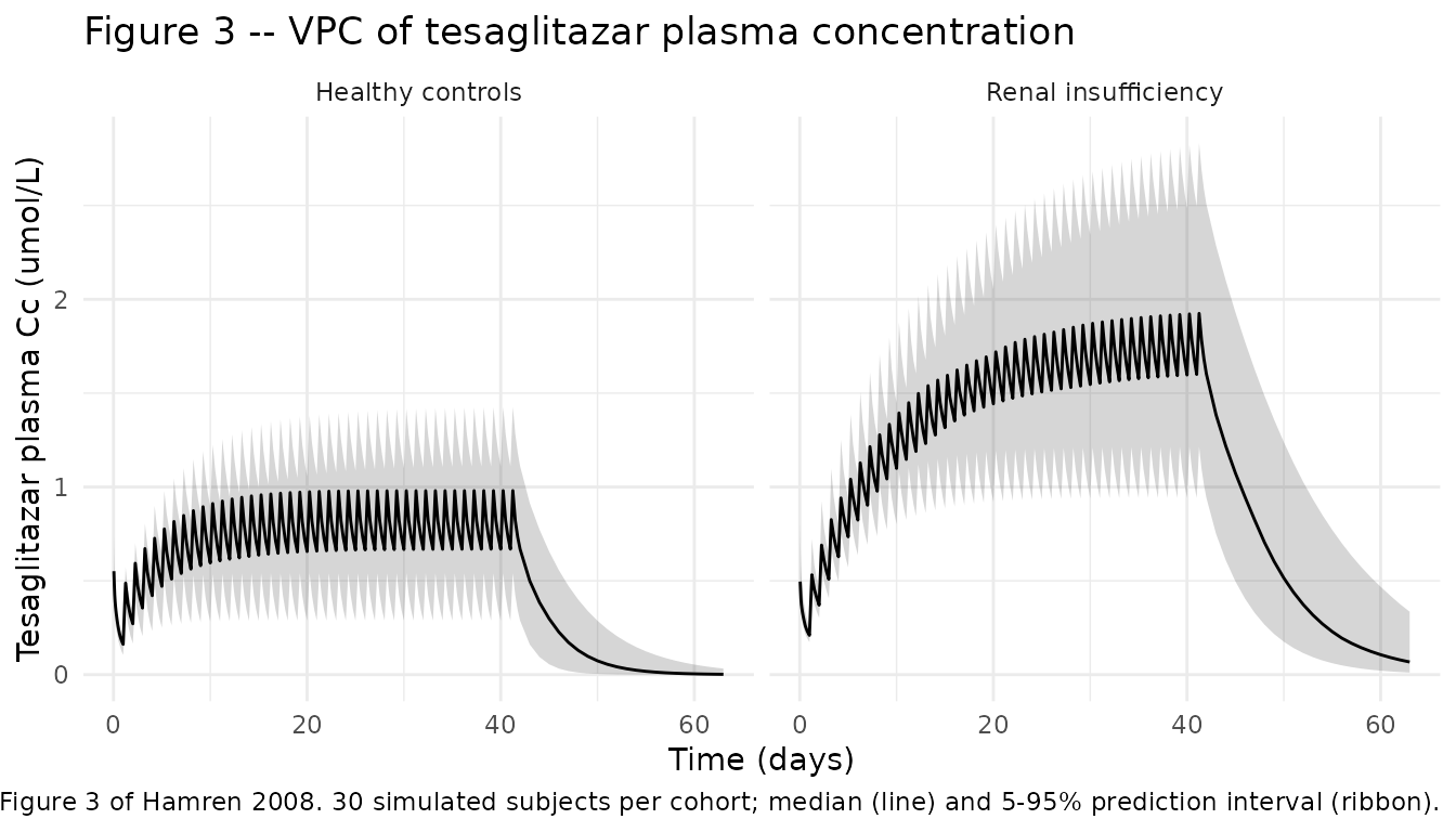

Replicate Figure 4 – acyl glucuronide plasma profile by cohort

Hamren 2008 Figure 4 shows the corresponding VPC for plasma acyl glucuronide. The renal-insufficiency cohort shows the saturable-renal-elimination feature (higher SS metabolite concentration than controls because Vmax is scaled by CRCL/76 = 32/76 = 0.42 in the IRF cohort vs 90/76 = 1.18 in controls):

sim |>
  dplyr::filter(time > 0) |>
  dplyr::group_by(time, cohort_label) |>
  dplyr::summarise(
    Q05 = quantile(Cc_gluc, 0.05, na.rm = TRUE),
    Q50 = quantile(Cc_gluc, 0.50, na.rm = TRUE),
    Q95 = quantile(Cc_gluc, 0.95, na.rm = TRUE),
    .groups = "drop"
  ) |>
  dplyr::mutate(time_days = time / 24) |>
  ggplot(aes(time_days, Q50)) +
  geom_ribbon(aes(ymin = Q05, ymax = Q95), alpha = 0.20) +
  geom_line() +
  facet_wrap(~ cohort_label) +
  scale_y_continuous(limits = c(0, NA)) +
  labs(
    x = "Time (days)",
    y = "Acyl glucuronide plasma Cc_gluc (umol/L)",
    title = "Figure 4 -- VPC of acyl glucuronide plasma concentration",
    caption = paste0(
      "Replicates Figure 4 of Hamren 2008. ",
      n_per_cohort, " simulated subjects per cohort; median (line) and ",
      "5-95% prediction interval (ribbon)."
    )
  ) +
  theme_minimal()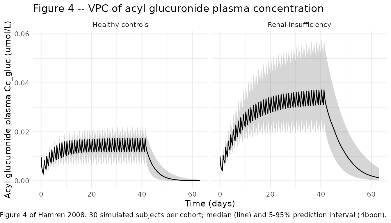

Typical-value steady-state trajectories

Typical-value (deterministic) plasma trajectories during the day-42 dosing interval highlight the renal-impairment-driven exposure increase the paper proposes as evidence for the interconversion mechanism:

ss_start <- 41 * 24
ss_end   <- 43 * 24

sim_typical |>
  dplyr::filter(time >= ss_start, time <= ss_end) |>
  dplyr::mutate(time_h = time - ss_start) |>
  tidyr::pivot_longer(c(Cc, Cc_gluc),
                      names_to = "analyte", values_to = "conc_umolL") |>
  dplyr::mutate(analyte = dplyr::recode(analyte,
    Cc      = "Tesaglitazar (parent)",
    Cc_gluc = "Acyl glucuronide (metabolite)"
  )) |>
  ggplot(aes(time_h, conc_umolL, colour = cohort_label)) +
  geom_line(linewidth = 0.8) +
  facet_wrap(~ analyte, scales = "free_y") +
  labs(
    x = "Hours into day 42 dosing interval",
    y = "Plasma concentration (umol/L)",
    colour = "Cohort",
    title = "Typical-value steady-state plasma profile, day 42",
    caption = "Deterministic single-subject typical-value simulation per cohort."
  ) +
  theme_minimal()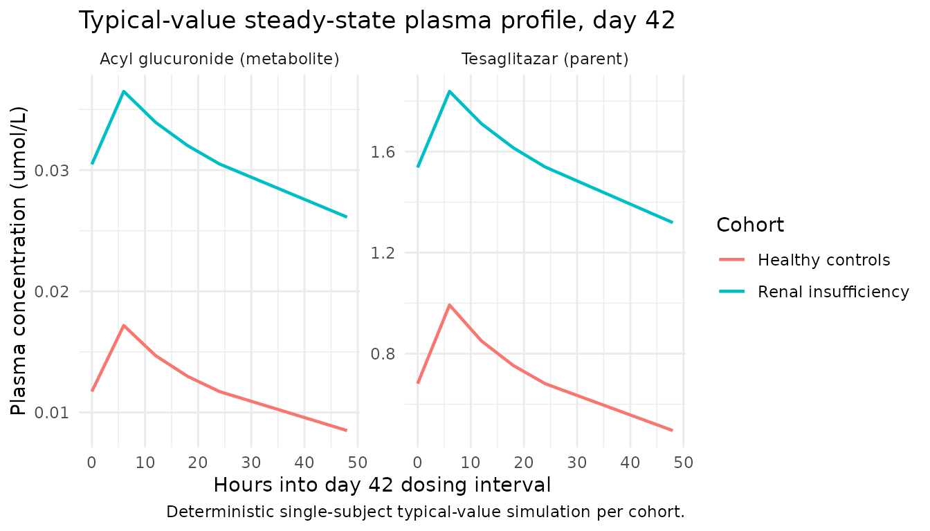

Replicate Table 3 – 24-hour urine amounts at steady state

Hamren 2008 Table 3 reports the 24-hour urine amounts of tesaglitazar and the acyl glucuronide at steady state (day 42), in umol, separately for the renal-insufficiency and healthy-control cohorts. The packaged model reproduces each cohort median below.

# Day 42 = the 42nd dose; the 42nd dose lands at time = 41*24 = 984 h.
# Urine accumulated between t = 984 (just before 42nd dose) and t = 1008
# is the 24-hour urine sample.
t_pre  <- 984
t_post <- 1008

# Extract cumulative urine state values bracketing the 24-h SS interval.
urine_ss <- sim |>
  dplyr::filter(time %in% c(t_pre, t_post)) |>
  dplyr::select(id, cohort_label, time, urine, urine_gluc) |>
  tidyr::pivot_wider(
    id_cols     = c(id, cohort_label),
    names_from  = time,
    values_from = c(urine, urine_gluc)
  ) |>
  dplyr::mutate(
    tesa_ss_umol = .data[[paste0("urine_",      t_post)]] -
                   .data[[paste0("urine_",      t_pre)]],
    gluc_ss_umol = .data[[paste0("urine_gluc_", t_post)]] -
                   .data[[paste0("urine_gluc_", t_pre)]]
  )

urine_summary <- urine_ss |>
  dplyr::group_by(cohort_label) |>
  dplyr::summarise(
    tesa_median = median(tesa_ss_umol),
    tesa_q025   = quantile(tesa_ss_umol, 0.025),
    tesa_q975   = quantile(tesa_ss_umol, 0.975),
    gluc_median = median(gluc_ss_umol),
    gluc_q025   = quantile(gluc_ss_umol, 0.025),
    gluc_q975   = quantile(gluc_ss_umol, 0.975),
    .groups = "drop"
  )

knitr::kable(
  urine_summary,
  caption = paste0(
    "Simulated 24-hour urine amounts at steady state (day 42), umol. ",
    "Median (Q50) and 2.5-97.5% prediction interval across ", n_per_cohort,
    " subjects per cohort."
  ),
  digits  = 2
)

Simulated 24-hour urine amounts at steady state (day 42), umol. Median (Q50) and 2.5-97.5% prediction interval across 30 subjects per cohort.
cohort_label	tesa_median	tesa_q025	tesa_q975	gluc_median	gluc_q025	gluc_q975
Healthy controls	0.56	0.28	1.10	1.41	0.92	1.93
Renal insufficiency	0.61	0.30	1.07	0.91	0.60	1.10

The published Table 3 values for comparison (observed median, observed range, simulated median, simulated 95% PI):

published <- tibble::tribble(
  ~cohort_label,           ~analyte,           ~observed_median, ~observed_range, ~simulated_median_paper, ~simulated_95pi_paper,
  "Renal insufficiency",   "Tesaglitazar",     0.42,             "0.18-0.97",     0.52,                     "0.13-1.4",
  "Healthy controls",      "Tesaglitazar",     0.54,             "0.38-0.79",     0.54,                     "0.13-1.2",
  "Renal insufficiency",   "Acyl glucuronide", 0.82,             "0.21-1.8",      0.80,                     "0.26-1.9",
  "Healthy controls",      "Acyl glucuronide", 1.4,              "0.54-1.7",      1.4,                      "0.62-2.4"
)

knitr::kable(
  published,
  caption = paste0(
    "Hamren 2008 Table 3 reference values: observed cohort medians + ranges, ",
    "and the published model's simulated medians + 95% prediction intervals ",
    "from the 1000-replicate posterior predictive check."
  )
)

Hamren 2008 Table 3 reference values: observed cohort medians + ranges, and the published model’s simulated medians + 95% prediction intervals from the 1000-replicate posterior predictive check.
cohort_label	analyte	observed_median	observed_range	simulated_median_paper	simulated_95pi_paper
Renal insufficiency	Tesaglitazar	0.42	0.18-0.97	0.52	0.13-1.4
Healthy controls	Tesaglitazar	0.54	0.38-0.79	0.54	0.13-1.2
Renal insufficiency	Acyl glucuronide	0.82	0.21-1.8	0.80	0.26-1.9
Healthy controls	Acyl glucuronide	1.40	0.54-1.7	1.40	0.62-2.4

PKNCA validation – steady-state Cmax / Cmin / AUC over the day-42 dosing interval

The source paper does not report a tabulated NCA summary (Cmax, AUC0-tau, half-life) per cohort; the model is validated against VPCs (Figures 3-4) and Table 3 urine amounts above. The PKNCA computation below derives steady-state Cmax, Cmin, AUC0-tau, and average concentration over the day-42 dose interval [t = 984, t = 1008] for both cohorts as a descriptive supplement.

sim_nca <- sim |>
  dplyr::filter(!is.na(Cc)) |>
  dplyr::select(id, time, Cc, cohort_label)

# Defensive time-zero record (per pknca-recipes.md): guarantee a Cc = 0
# row at t = 0 per (id, cohort_label) so PKNCA can anchor AUC.
sim_nca <- dplyr::bind_rows(
  sim_nca,
  sim_nca |>
    dplyr::distinct(id, cohort_label) |>
    dplyr::mutate(time = 0, Cc = 0)
) |>
  dplyr::distinct(id, cohort_label, time, .keep_all = TRUE) |>
  dplyr::arrange(id, cohort_label, time)

conc_obj <- PKNCA::PKNCAconc(
  sim_nca,
  Cc ~ time | cohort_label + id,
  concu = "umol/L",
  timeu = "h"
)

dose_df <- events |>
  dplyr::filter(evid == 1L) |>
  dplyr::select(id, time, amt, cohort_label)

dose_obj <- PKNCA::PKNCAdose(
  dose_df,
  amt ~ time | cohort_label + id,
  doseu = "umol"
)

intervals <- data.frame(
  start    = 984,
  end      = 1008,
  cmax     = TRUE,
  cmin     = TRUE,
  tmax     = TRUE,
  auclast  = TRUE,
  cav      = TRUE
)

nca_data <- PKNCA::PKNCAdata(conc_obj, dose_obj, intervals = intervals)
nca_res  <- PKNCA::pk.nca(nca_data)

nca_tbl <- as.data.frame(nca_res$result) |>
  dplyr::select(cohort_label, id, PPTESTCD, PPORRES) |>
  tidyr::pivot_wider(names_from = PPTESTCD, values_from = PPORRES) |>
  dplyr::group_by(cohort_label) |>
  dplyr::summarise(
    cmax_median    = median(cmax,    na.rm = TRUE),
    cmin_median    = median(cmin,    na.rm = TRUE),
    tmax_median    = median(tmax,    na.rm = TRUE),
    auclast_median = median(auclast, na.rm = TRUE),
    cav_median     = median(cav,     na.rm = TRUE),
    .groups = "drop"
  )

knitr::kable(
  nca_tbl,
  caption = paste0(
    "PKNCA-derived steady-state (day 42) tesaglitazar plasma NCA parameters ",
    "per cohort; medians across ", n_per_cohort, " simulated subjects per ",
    "cohort. Cmax / Cmin in umol/L, AUClast in umol*h/L, tmax in hours."
  ),
  digits = 3
)

PKNCA-derived steady-state (day 42) tesaglitazar plasma NCA parameters per cohort; medians across 30 simulated subjects per cohort. Cmax / Cmin in umol/L, AUClast in umol*h/L, tmax in hours.
cohort_label	cmax_median	cmin_median	tmax_median	auclast_median	cav_median
Healthy controls	0.981	0.669	6	18.997	0.792
Renal insufficiency	1.925	1.600	6	41.934	1.747

The renal-insufficiency cohort shows higher SS Cmax / AUC than the controls, reproducing the increased tesaglitazar exposure in IRF that the source paper attributes to the interconversion mechanism.

Assumptions and deviations

Parametric IIV diagonal carried; nonparametric covariance not portable. The source paper’s final published fit used a NONPARAMETRIC variance-covariance matrix (Results ‘Pharmacokinetic analysis’) with non-zero off-diagonal correlations (Table 2 footnote: CLmt-Vpt = 0.68, CLmt-Vct = -0.43, CLmt-CLnrm = -0.63, CLrt-Vct = -0.44, Km-Vct = -0.46, CLnrm-Vpt = 0.47). This packaged model uses the parametric diagonal CV% values from Table 2 (CLmt 18%, CLrt 20%, Vct 39%, Vpt 16%, Km 37%, CLnrm 54%) as a log-normal IIV diagonal because (a) the nonparametric matrix is not a Gaussian parameter set that nlmixr2 / rxode2 can encode directly and (b) the parametric form is the standard portable shape for a packaged model. Hamren 2008 reports that the nonparametric method improved predictive performance over the parametric matrix (modest overestimation of IIV variability in plasma); virtual cohorts simulated from this packaged model are therefore expected to show slightly wider 95% PIs than the source paper’s Figures 3-4. Users wanting the nonparametric matrix can approximate it by sampling etas from a multivariate normal with the parametric variances on the diagonal and the Table 2 footnote correlations on the off-diagonals.
Probenecid effect encoded as two separate parameters with the same value. Hamren 2008 Table 2 reports a single shared theta for the probenecid effect that was applied jointly to CLrt and Vmax during NONMEM estimation (Methods ‘Pharmacokinetic modelling’). The packaged model carries e_probenecid_cl_renal and e_probenecid_vmax_gluc as two separate parameters initialised to the same -0.75 value so that each covariate-parameter pair follows the canonical e_<cov>_<param> naming. Numerically identical to the source paper’s encoding for any simulation use case; the deviation is structural only.
kint (paper) -> kicv (canonical) rename for the interconversion rate constant. Hamren 2008 names the gut-hydrolysis-and-parent- reabsorption rate constant kint = 0.79 1/h. nlmixr2lib already has a canonical kint for TMDD complex internalisation, which is a mechanistically distinct concept. The interconversion rate is renamed to the canonical kicv (registered alongside this extraction in inst/references/parameter-names.md) so the two roles are kept semantically distinct. The packaged value of kicv is unchanged from Hamren’s kint = 0.79 1/h.
CLiohexol encoded under CRCL with broadened scope. The Hamren 2008 Methods describes renal function assessment by plasma iohexol clearance, the clinical gold-standard tracer-measured glomerular filtration rate. The CRCL canonical was originally limited to creatinine-based renal function (MDRD / CKD-EPI eGFR or measured CrCl BSA-normalised) and was extended in inst/references/covariate-columns.md to cover both creatinine-based and tracer-measured GFR (iohexol, inulin, 99mTc-DTPA, 51Cr-EDTA), per the standing decision recorded in this task’s sidecar response 001 (2026-06-17). The packaged covariateData entry records source_name = 'CLiohexol' and flags the iohexol-tracer assay in notes.
FU registered as a new canonical covariate column. Per-subject fraction unbound of the parent drug in plasma (measured by ultrafiltration) was not in the covariate register before this extraction. The FU canonical was added to inst/references/covariate-columns.md (in the protein-binding cluster after TPRO) with Hamren 2008 as the founding example, per the operator decision in sidecar response 001.
kbm and kicv registered as new canonical paper-mechanistic parameters. Hamren 2008’s biliary-excretion rate constant kbm and interconversion rate constant (renamed kicv to avoid the TMDD kint clash) were not in inst/references/parameter-names.md before this extraction. Both were registered as new canonical paper-named parameters (under the kint cluster) with Hamren 2008 as the founding example, per the operator decision in sidecar response 001.
Per-subject FU and SEXF replaced with cohort-typical values in the virtual cohort. The source paper records subject-level FU measurements (range 0.06-0.2%; cohort median 0.1% imputed for three subjects with missing values) and subject-level SEXF (cohort medians reported in Table 1). The virtual-cohort tables above hold FU at the per-cohort median (0.11% IRF, 0.09% controls) and SEXF at a per-cohort fraction (0.30 IRF, 0.40 controls) – so the simulated SEXF column is a real-valued probability rather than a hard 0/1 indicator, which the linear (1 + e_sexf_cl_renal * SEXF) form accepts because the coefficient is small (-0.31). For a hard 0/1 cohort, redefine SEXF per-subject (binomial draw with the cohort median p) rather than per-cohort.
WT held constant per cohort at Table 1 median. Body weight is time-fixed at the per-cohort median (84 kg IRF, 75 kg controls). Subject-level variability across the published WT range (62-107 kg IRF, 60-97 kg controls) is not simulated here because the WT covariate effect on Vct and Vpt is small (e_wt_vc_vp = 0.0094 per kg over 80 kg, so the realised effect is approximately +/-25% across the cohort range and contributes a minor share of the plasma variability seen in Figures 3-4 relative to the IIV on CLmt, CLrt, Vct, Vpt, Km, and CLnrm).
Tesaglitazar molecular weight assumed at 408.45 g/mol. The source paper expresses metabolite parameters in molar units (Vmax in umol/h, Km in umol/L) without stating the parent’s molecular weight explicitly. The dose-to-amount conversion in the virtual cohort (dose_umol = 1.0 mg / 408.45 g/mol * 1000 = 2.4483 umol per 1 mg tablet) uses 408.45 g/mol, derived from the published structural formula C20H22O7S (Figure 1 of the source). Users with a different tesaglitazar MW reference can rescale dose_umol accordingly.
No errata identified. A PubMed search for Hamren 2008 tesaglitazar erratum and a BJCP corrections-feed scan returned no corrections as of the extraction date (2026-06-20).
No NONMEM control stream on disk. The source PDF + its trimmed markdown companion are the only artefacts available; no .mod / .ctl / .lst is supplied. All parameter values are sourced from Table 2 of the main publication. The ADVAN6 (general nonlinear kinetics) subroutine was used in the original NONMEM VI fit (Methods ‘Data analysis’).