Vancomycin (Yoon 2023)

Model and source

• Citation: Yoon S, Guk J, Lee S-G, Chae D, Kim J-H, Park K. Model-informed precision dosing in vancomycin treatment. Front Pharmacol. 2023;14:1252757. doi:10.3389/fphar.2023.1252757
• Description: Joint population PK/PD model for intravenous vancomycin in Korean hospitalised adults and children (Yoon 2023). Two-compartment PK with allometric scaling on CL/Q (0.75) and V/Vp (1) referenced to 70 kg; clearance is further scaled by a renal-function factor built from a creatinine-production-rate model that declines with age above 30 years and rises with age below it, by a sigmoid postmenstrual-age maturation factor, and by an exponential blood-urea-nitrogen effect together with proportional shifts for female sex, diabetes and renal disease. Vancomycin-induced nephrotoxicity is carried as a first-order exponential decline of creatinine clearance with time on therapy. The PD layer describes C-reactive protein with a proliferation compartment feeding two transit compartments and a circulating CRP compartment, whose production is stimulated linearly by a latent disease-severity state; severity grows first-order and is suppressed by cumulative vancomycin AUC, and the transit rate constant increases additively in patients with pneumonia. Vancomycin concentrations carry separate combined proportional-plus-additive residual errors for peak and trough samples.
• Article: https://doi.org/10.3389/fphar.2023.1252757

Yoon 2023 is a model-informed precision dosing (MIPD) analysis of therapeutic drug monitoring records from Severance Hospital, Seoul. It contributes two coupled layers that are extracted here as a single model file, because the PD layer is driven by the cumulative AUC of the PK layer and the two were fitted as one system:

• a two-compartment popPK model for intravenous vancomycin spanning neonates to the elderly, whose clearance carries an explicit renal-function submodel, a postmenstrual-age maturation factor, and a nephrotoxicity term that lets creatinine clearance fall with time on therapy; and
• a semi-mechanistic CRP model in which a proliferation compartment feeds two transit compartments and a circulating CRP compartment, with production stimulated by a latent disease-severity state that vancomycin exposure suppresses.

Population

The analysis is retrospective, drawn from the electronic medical records of 542 hospitalised patients who received intravenous vancomycin and underwent therapeutic drug monitoring (Yoon 2023 Table 1). The cohort spans the entire age range: 22 patients were under 4 years old, 18 were aged 4-19, and 502 were adults, with a median age of 60 years (range 0-93) and a median weight of 59 kg (range 2.6-106). 41.1% were female. 1,526 vancomycin concentrations were available, roughly three per patient, drawn as peak (end-of-infusion) and trough (start-of-infusion) pairs. Median serum creatinine was 0.7 mg/dL (range 0.2-12.9) and median BUN 15.25 mg/dL (range 1.5-141.5). Comorbidity was common: hypertension 52.4%, cardiovascular disease 47.2%, diabetes 28.4%, haematological malignancy 22.5%, sepsis 17.5% and renal disease 27.1% (pooled across acute kidney disease 9.04%, chronic kidney disease 8.86% and other 9.23%).

128 of those patients also had CRP measurements and form the PD dataset (Table 2): 845 CRP observations, median age 63 years, median weight 57.15 kg, 38.3% female, median CRP 73 mg/L (range 0.4-479.2), and pneumonia in 32.0%. Vancomycin was given at 500-1500 mg per dose with intervals from 6 to 24 h. Mean length of stay was 20 days, with one patient hospitalised for 113 days because of a secondary pneumonia.

The same information is available programmatically via the model’s population metadata (readModelDb("Yoon_2023_vancomycin")()$population).

Source trace

Every ini() entry carries an in-file comment naming its source location in inst/modeldb/specificDrugs/Yoon_2023_vancomycin.R. The table below collects them for review. Equation numbers refer to the display equations of the published article, recovered from the MathML in the PubMed Central full-text XML; the PDF-derived markdown renders them as formula-not-decoded.

Equation / parameter	Value	Source location
TVV = thetaV * (WT/70) * COVV	n/a	Eq. 1 / Eq. 3
TVCL = thetaCL * (WT/70)^0.75 * Fren * Fmat * COVCL	n/a	Eq. 2 / Eq. 4
Fren = (CLCr / CLCr_TV)^lambda	n/a	Eq. 5
CLCr = RCr / Cr * exp(-ktox * t)	n/a	Eq. 6
RCr = 64.2 * exp(kCr * (age - 30))	n/a	Eq. 7
Fmat = PMA^gamma / (PMA50^gamma + PMA^gamma)	n/a	Eq. 8
COVCL = exp(kBUN*(BUN-15)) * (1+thetaFEM*FEM) * (1+thetaDM*DM) * (1+thetaREN*REN)	n/a	Eq. 15
COVV = exp(kV * (age - 40))	n/a	Eq. 16
d/dt(Prol) = Kin*(1 + SCRP*D) - Kout*Prol	n/a	Eq. 9
d/dt(Tran1) = ktr*(Prol - Tran1)	n/a	Eq. 10
d/dt(Tran2) = ktr*(Tran1 - Tran2)	n/a	Eq. 11
d/dt(CRP) = ktr*Tran2 - kCRP*CRP	n/a	Eq. 12
d/dt(D) = kD * D * (1 - EDrug)	n/a	Eq. 13
EDrug = alpha * AUC	n/a	Eq. 14
ktr = theta_ktr + thetaPNE * PNE	n/a	Eq. 17 (Results 3.3)
lcl (thetaCL)	4.32 L/h	Table 3
lvc (thetaV)	38.6 L	Table 3
lq (thetaQ)	3.93 L/h	Table 3
lvp (thetaV2)	66.8 L	Table 3
e_wt_cl_q	0.75 (fixed)	Eq. 2 exponent
e_wt_vc_vp	1 (fixed)	Eq. 1 exponent
kcr_agege30	-0.0127 /yr	Table 3
kcr_agelt30	0.0193 /yr	Table 3
e_crcl_cl (lambda)	0.655	Table 3
pma50_cl	43.9 weeks	Table 3
h_pma_cl (gamma)	2.08	Table 3
ktox	0.00598 /day	Table 3
e_age_vc (kV)	0.00957 /yr	Table 3
e_bun_cl (kBUN)	-0.00874 dL/mg	Table 3
e_dis_renal_cl (thetaREN)	-0.237	Table 3
e_sexf_cl (thetaFEM)	-0.199	Table 3
e_dis_diab_cl (thetaDM)	-0.151	Table 3
etalcl	CV 29.1%	Table 3
etalvp	CV 101%	Table 3
propSd_Cctrough / addSd_Cctrough	17.8% / 0.956 mg/L	Table 3
propSd_Ccpeak / addSd_Ccpeak	11.0% / 4.47 mg/L	Table 3
lktr (theta_ktr)	0.0129 /h	Table 4
e_dis_pneumonia_ktr (thetaPNE)	0.0058 /h	Table 4
lkout (kCRP)	0.0365 /h (fixed)	Results 3.3 text (Table 4 prints 0.365; see Errata)
lrbase (CRP0)	110 mg/L	Table 4
lkdis (kD)	0.00192 /h	Table 4
e_auc_kdis (alpha)	0.000239 L/(mg*h)	Table 4
scrp (SCRP)	102	Table 4
etalkdis	CV 147.6%	Table 4
etalrbase	CV 107.2%	Table 4
propSd_crp	CV 54.9%	Table 4

mod <- readModelDb("Yoon_2023_vancomycin")
ui  <- rxode2::rxode(mod)
#> ℹ parameter labels from comments will be replaced by 'label()'

# Typical-value form for the deterministic replications below. zeroRe() sets
# every IIV variance to zero, which is sufficient on its own -- rxSolve reports
# "omega/sigma items treated as zero" for each eta and returns the typical-value
# trajectory. An earlier version of this file also passed `omega = NA` at solve
# time, on the theory that rxSolve would otherwise reuse an omega from a
# previous call. That is not so for a zeroRe()d model, and the argument was
# actively harmful: combined with a multi-subject `params` it triggers an
# out-of-bounds read in rxode2 5.1.6. See the table5 solve for the measurements.
mod_typ <- rxode2::zeroRe(mod)
#> ℹ parameter labels from comments will be replaced by 'label()'

Deterministic parameter identities

Three published quantities are exact algebraic consequences of the estimates in Tables 3 and 4, so they are checked directly rather than by simulation. They are deterministic, so the tolerances here are tight on purpose.

th <- ui$theta

ktr_none <- exp(th[["lktr"]])
ktr_pne  <- exp(th[["lktr"]]) + th[["e_dis_pneumonia_ktr"]]

identities <- tibble::tibble(
  Quantity = c(
    "Mean transit time, no pneumonia (days)",
    "Mean transit time, pneumonia (days)",
    "CRP half-life (h)",
    "Dose reduction, renal disease (%)",
    "Dose reduction, diabetes (%)",
    "Dose reduction, female (%)"
  ),
  Published = c(9.62, 6.65, 19, 23, 15, 20),
  Model = c(
    3 / ktr_none / 24,          # three compartments upstream of CRP: prol, transit1, transit2
    3 / ktr_pne / 24,
    log(2) / exp(th[["lkout"]]),
    -100 * th[["e_dis_renal_cl"]],
    -100 * th[["e_dis_diab_cl"]],
    -100 * th[["e_sexf_cl"]]
  )
) |>
  dplyr::mutate(`Difference (%)` = 100 * (Model - Published) / Published)

identities |>
  dplyr::rename("Model value" = Model, "Published value" = Published) |>
  knitr::kable(digits = 2, caption = "Published quantities recovered algebraically from the packaged parameters.")

Published quantities recovered algebraically from the packaged parameters.

Quantity	Published value	Model value	Difference (%)
Mean transit time, no pneumonia (days)	9.62	9.69	0.73
Mean transit time, pneumonia (days)	6.65	6.68	0.52
CRP half-life (h)	19.00	18.99	-0.05
Dose reduction, renal disease (%)	23.00	23.70	3.04
Dose reduction, diabetes (%)	15.00	15.10	0.67
Dose reduction, female (%)	20.00	19.90	-0.50

# All six are algebra on fixed numbers -- no simulation, no cohort, no RNG.
# The transit-time pair also confirms the chain length (three compartments feed
# CRP) and that the pneumonia effect on ktr is ADDITIVE: a multiplicative
# reading would give 9.62/(1+0.0058) = 9.57 days, not 6.65.
stopifnot(max(abs(identities$`Difference (%)`)) < 3.5)

Reproducing the published optimal-dose tables

Yoon 2023 Table 5 is the paper’s principal output: for each combination of age, weight, serum creatinine and BUN, the daily dose (given four times a day) whose steady-state trough sits closest to the adult target of 15 mg/L, searched on a 0.2 g/day grid. Reproducing that table exercises the whole PK layer at once – the structural parameters, the allometry, the renal-function submodel and every covariate effect.

Because the model is linear in dose, the trough at any dose is the trough at 1 g/day scaled by the dose ratio, so one solve per covariate combination suffices.

# Deterministic typical-value covariate grid, not a stochastic cohort: each row
# is one covariate combination from Yoon 2023 Table 5, solved with IIV zeroed.
table5_grid <- tidyr::crossing(
  AGE   = c(20, 40, 60, 80),
  WT    = c(40, 50, 60, 70, 80, 90),
  CREAT = c(0.5, 1.0, 1.5, 2.0, 2.5),
  BUN   = c(10, 20, 30, 40)
) |>
  dplyr::mutate(
    id            = dplyr::row_number(),
    PAGE          = AGE * 52.18 + 40,   # postmenstrual age in weeks; Fmat ~ 1 for adults
    SEXF          = 0,                  # Table 5 is the male, non-diabetic,
    DIS_DIAB      = 0,                  # no-renal-disease reference cell; the
    DIS_RENAL     = 0,                  # footnote gives the shifts for the rest
    DIS_PNEUMONIA = 0
  )

nrow(table5_grid)
#> [1] 480

t_ss <- 24 * 10   # trough sampled after ten days of q6h dosing

ev_table5 <- table5_grid |>
  dplyr::select(id) |>
  tidyr::crossing(tibble::tibble(time = 0)) |>
  dplyr::transmute(id, time, amt = 250, evid = 1L, dur = 1, ii = 6, addl = t_ss / 6 - 1,
                   cmt = "central", dvid = NA_integer_) |>
  dplyr::bind_rows(
    table5_grid |> dplyr::select(id) |>
      dplyr::mutate(time = t_ss, amt = NA_real_, evid = 0L, dur = NA_real_,
                    ii = NA_real_, addl = NA_real_, cmt = "central", dvid = 1L)
  ) |>
  dplyr::arrange(id, time, dplyr::desc(evid))

# The model declares three endpoints (Cctrough, Ccpeak, crp), so every
# observation row must carry a dvid. dvid = 1 selects Cctrough; rxSolve returns
# every other observable (Cc, Ccpeak, crp, severity, ...) as a column anyway.
sim_table5 <- rxode2::rxSolve(
  mod_typ,
  events = ev_table5,
  params = table5_grid |>
    dplyr::select(id, AGE, WT, CREAT, BUN, PAGE, SEXF, DIS_DIAB, DIS_RENAL, DIS_PNEUMONIA),
  # NO `omega = NA` here, deliberately. `mod_typ` is already `zeroRe()`d, so the
  # etas are zero either way -- but passing `omega = NA` alongside a
  # multi-subject `params` makes rxode2 5.1.6 index a length-1 vector once per
  # extra subject, emitting 479 "subscript out of bounds (index i >= vector
  # size 1)" warnings on this 480-row grid. That out-of-bounds read CORRUPTS
  # results: 23 of the 480 troughs come back attached to the wrong covariate
  # row (max difference 33.98 mg/L), and some runs return `Cc = NA` outright,
  # which is what intermittently failed the assertion below.
  #
  # An earlier pass misread that as solver stiffness and raised `maxsteps` to
  # 1e5. That was wrong: the warning count and the corrupted values are
  # identical at the default ceiling and at 1e5, so the step limit was never
  # involved. It masked the failure once by perturbing the run, which is why it
  # looked load-sensitive. Dropping the redundant argument is the actual fix and
  # `maxsteps` goes with it.
  useLinCmt = FALSE,      # ODE -> linCmt auto-conversion breaks multi-endpoint dvid mapping
  returnType = "data.frame"
) |>
  dplyr::filter(time == t_ss)
#> ℹ omega/sigma items treated as zero: 'etalcl', 'etalvp', 'etalkdis', 'etalrbase'
#> Warning: multi-subject simulation without without 'omega'

# 250 mg q6h = 1 g/day, so this trough corresponds to a 1 g/day regimen.
table5_cmp <- table5_grid |>
  dplyr::left_join(
    sim_table5 |> dplyr::transmute(id = as.integer(as.character(id)), trough_1g = Cc),
    by = "id"
  ) |>
  dplyr::mutate(
    dose_exact = 15 / trough_1g,                    # linear in dose
    dose_model = round(dose_exact / 0.2) * 0.2      # the paper's 0.2 g/day search grid
  )

stopifnot(nrow(table5_cmp) == 480, all(is.finite(table5_cmp$dose_model)))

The published table is transcribed below, in the same age x weight x creatinine x BUN order.

published_table5 <- tibble::tribble(
  ~AGE, ~WT, ~doses,
  20, 40, c(2.2,2,1.8,1.6, 1.2,1.2,1,1, 1,0.8,0.8,0.6, 0.8,0.6,0.6,0.6, 0.6,0.6,0.6,0.6),
  20, 50, c(2.6,2.4,2,1.8, 1.4,1.4,1.2,1, 1,1,1,0.8, 0.8,0.8,0.8,0.6, 0.8,0.8,0.6,0.6),
  20, 60, c(3,2.6,2.4,2.2, 1.6,1.6,1.4,1.2, 1.2,1.2,1,1, 1,1,0.8,0.8, 0.8,0.8,0.8,0.8),
  20, 70, c(3.2,3,2.6,2.4, 1.8,1.6,1.6,1.4, 1.4,1.2,1.2,1, 1.2,1,1,1, 1,1,0.8,0.8),
  20, 80, c(3.6,3.2,2.8,2.6, 2,1.8,1.6,1.6, 1.6,1.4,1.2,1.2, 1.2,1.2,1,1, 1.2,1,1,0.8),
  20, 90, c(4,3.4,3.2,2.8, 2.2,2,1.8,1.6, 1.6,1.6,1.4,1.2, 1.4,1.2,1.2,1, 1.2,1.2,1,1),
  40, 40, c(2.2,2,1.8,1.6, 1.2,1.2,1,1, 1,0.8,0.8,0.8, 0.8,0.8,0.6,0.6, 0.6,0.6,0.6,0.6),
  40, 50, c(2.6,2.4,2,1.8, 1.4,1.4,1.2,1.2, 1.2,1,1,0.8, 1,0.8,0.8,0.8, 0.8,0.8,0.6,0.6),
  40, 60, c(3,2.6,2.4,2.2, 1.6,1.6,1.4,1.2, 1.2,1.2,1,1, 1,1,0.8,0.8, 1,0.8,0.8,0.8),
  40, 70, c(3.2,3,2.6,2.4, 1.8,1.8,1.6,1.4, 1.4,1.4,1.2,1, 1.2,1,1,1, 1,1,0.8,0.8),
  40, 80, c(3.6,3.2,2.8,2.6, 2,1.8,1.8,1.6, 1.6,1.4,1.4,1.2, 1.4,1.2,1.2,1, 1.2,1,1,1),
  40, 90, c(3.8,3.4,3.2,2.8, 2.2,2,1.8,1.8, 1.8,1.6,1.4,1.4, 1.4,1.4,1.2,1.2, 1.2,1.2,1,1),
  60, 40, c(1.8,1.6,1.4,1.2, 1,1,0.8,0.8, 0.8,0.8,0.6,0.6, 0.6,0.6,0.6,0.6, 0.6,0.6,0.4,0.4),
  60, 50, c(2,1.8,1.6,1.4, 1.2,1,1,1, 1,0.8,0.8,0.8, 0.8,0.8,0.6,0.6, 0.6,0.6,0.6,0.6),
  60, 60, c(2.2,2,1.8,1.6, 1.4,1.2,1.2,1, 1,1,1,0.8, 0.8,0.8,0.8,0.8, 0.8,0.8,0.6,0.6),
  60, 70, c(2.6,2.2,2,1.8, 1.6,1.4,1.2,1.2, 1.2,1,1,1, 1,1,0.8,0.8, 0.8,0.8,0.8,0.8),
  60, 80, c(2.8,2.6,2.2,2, 1.8,1.6,1.4,1.4, 1.4,1.2,1.2,1, 1.2,1,1,1, 1,1,0.8,0.8),
  60, 90, c(3,2.8,2.4,2.2, 1.8,1.8,1.6,1.4, 1.4,1.4,1.2,1.2, 1.2,1.2,1,1, 1,1,1,1),
  80, 40, c(1.4,1.2,1.2,1, 0.8,0.8,0.8,0.6, 0.6,0.6,0.6,0.6, 0.6,0.6,0.4,0.4, 0.6,0.4,0.4,0.4),
  80, 50, c(1.6,1.4,1.4,1.2, 1,1,0.8,0.8, 0.8,0.8,0.6,0.6, 0.6,0.6,0.6,0.6, 0.6,0.6,0.6,0.6),
  80, 60, c(1.8,1.6,1.6,1.4, 1.2,1,1,1, 1,0.8,0.8,0.8, 0.8,0.8,0.6,0.6, 0.8,0.6,0.6,0.6),
  80, 70, c(2,1.8,1.6,1.6, 1.2,1.2,1.2,1, 1,1,0.8,0.8, 0.8,0.8,0.8,0.8, 0.8,0.8,0.8,0.6),
  80, 80, c(2.2,2,1.8,1.8, 1.4,1.4,1.2,1.2, 1.2,1,1,1, 1,1,0.8,0.8, 0.8,0.8,0.8,0.8),
  80, 90, c(2.4,2.2,2,1.8, 1.6,1.4,1.4,1.2, 1.2,1.2,1.2,1, 1,1,1,1, 1,1,1,0.8)
) |>
  dplyr::mutate(
    # Table 5 varies BUN fastest within each creatinine block.
    cell = lapply(doses, function(d) {
      tidyr::crossing(CREAT = c(0.5, 1.0, 1.5, 2.0, 2.5), BUN = c(10, 20, 30, 40)) |>
        dplyr::arrange(CREAT, BUN) |>
        dplyr::mutate(dose_published = d)
    })
  ) |>
  dplyr::select(AGE, WT, cell) |>
  tidyr::unnest(cell)

stopifnot(nrow(published_table5) == 480)

table5_final <- table5_cmp |>
  dplyr::inner_join(published_table5, by = c("AGE", "WT", "CREAT", "BUN")) |>
  dplyr::mutate(
    step_error = round((dose_model - dose_published) / 0.2)
  )
stopifnot(nrow(table5_final) == 480)

agreement <- tibble::tibble(
  Metric = c(
    "Cells reproduced exactly (%)",
    "Cells within one 0.2 g/day grid step (%)",
    "Median model/published dose ratio",
    "Median absolute difference (g/day)"
  ),
  Value = c(
    100 * mean(table5_final$step_error == 0),
    100 * mean(abs(table5_final$step_error) <= 1),
    median(table5_final$dose_exact / table5_final$dose_published),
    median(abs(table5_final$dose_model - table5_final$dose_published))
  )
)
knitr::kable(agreement, digits = 3,
             caption = "Agreement with the 480 published adult optimal doses of Yoon 2023 Table 5.")

Agreement with the 480 published adult optimal doses of Yoon 2023 Table 5.

Metric	Value
Cells reproduced exactly (%)	54.375
Cells within one 0.2 g/day grid step (%)	99.792
Median model/published dose ratio	0.916
Median absolute difference (g/day)	0.000

# The grid is deterministic (IIV zeroed), so these are not cohort statistics and
# do not vary with solver thread count. The bounds below still leave room for
# the two things the paper does not pin down -- the infusion duration and the
# exact steady-state day at which the trough was read -- both of which move the
# required dose by a few percent.
stopifnot(
  mean(abs(table5_final$step_error) <= 1) > 0.90,
  abs(median(table5_final$dose_exact / table5_final$dose_published) - 1) < 0.12
)

table5_final |>
  ggplot(aes(dose_published, dose_exact, colour = factor(CREAT))) +
  geom_abline(slope = 1, intercept = 0, linetype = "dashed") +
  geom_jitter(width = 0.03, height = 0, alpha = 0.6) +
  labs(x = "Published optimal dose (g/day)", y = "Model-required dose (g/day)",
       colour = "Creatinine\n(mg/dL)",
       title = "Reproducing Yoon 2023 Table 5",
       caption = "Each point is one of the 480 published adult covariate cells.")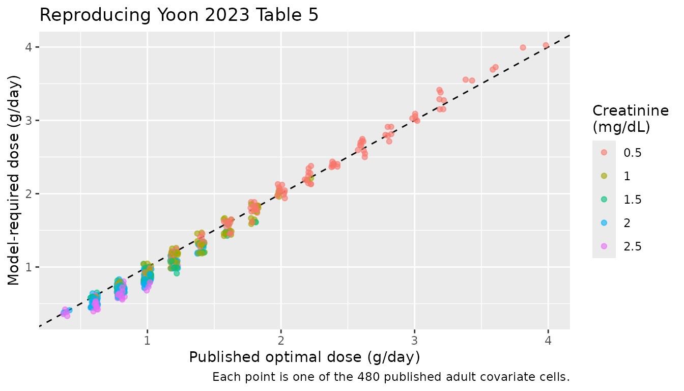

The published table also states the direction of every covariate trend, which the model reproduces:

trend <- function(df, var) {
  s <- df |> dplyr::group_by(.data[[var]]) |>
    dplyr::summarise(dose = median(dose_exact), .groups = "drop") |>
    dplyr::arrange(.data[[var]])
  s$dose
}
wt_trend    <- trend(table5_final, "WT")
creat_trend <- trend(table5_final, "CREAT")
bun_trend   <- trend(table5_final, "BUN")

# Yoon 2023 Results 3.4: "the optimal dose increased with weight, while it
# decreased with Cr and BUN levels. Regarding age, the dose exhibited an upward
# trend with age until 40, followed by a subsequent decrease."
age_trend <- trend(table5_final, "AGE")

tibble::tibble(
  Claim = c("Dose increases with weight",
            "Dose decreases with creatinine",
            "Dose decreases with BUN",
            "Dose peaks at age 40, then falls"),
  Reproduced = c(
    wt_trend[length(wt_trend)] > wt_trend[1],
    creat_trend[length(creat_trend)] < creat_trend[1],
    bun_trend[length(bun_trend)] < bun_trend[1],
    which.max(age_trend) == 2L
  )
) |>
  knitr::kable(caption = "Covariate trends stated in Yoon 2023 Results 3.4.")

Covariate trends stated in Yoon 2023 Results 3.4.

Claim	Reproduced
Dose increases with weight	TRUE
Dose decreases with creatinine	TRUE
Dose decreases with BUN	TRUE
Dose peaks at age 40, then falls	TRUE

stopifnot(
  wt_trend[length(wt_trend)] > wt_trend[1],
  creat_trend[length(creat_trend)] < creat_trend[1],
  bun_trend[length(bun_trend)] < bun_trend[1],
  which.max(age_trend) == 2L
)

Replicating Figure 6: the CRP time course

Figure 6 shows the simulated CRP profile by dose (panel A) and by pneumonia status (panel B) for a typical patient. Both panels start at CRP0 = 110 mg/L, fall steeply over the first ~150 h to a plateau, show a slow secondary rise as disease severity grows, and then decline as cumulative vancomycin exposure takes over.

# Typical patient of the PD cohort (Yoon 2023 Table 2 medians).
pd_typical <- tibble::tibble(
  AGE = 63, WT = 57, CREAT = 0.79, BUN = 18.05,
  PAGE = 63 * 52.18 + 40, SEXF = 0, DIS_DIAB = 0, DIS_RENAL = 0
)

tmax_pd <- 1250
base_daily_g <- 1.2   # the model-recommended dose for this covariate set, from
                      # the Table 5 reproduction above (age 60, WT 60, Cr ~1, BUN ~20)

fig6_arms <- dplyr::bind_rows(
  tibble::tibble(arm = c("0.5 times the dose", "recommended dose",
                         "1.5 times the dose", "2.0 times the dose"),
                 mult = c(0.5, 1, 1.5, 2), DIS_PNEUMONIA = 0, panel = "A: dose"),
  tibble::tibble(arm = c("no pneumonia", "pneumonia"),
                 mult = c(1, 1), DIS_PNEUMONIA = c(0, 1), panel = "B: pneumonia")
) |>
  dplyr::mutate(id = dplyr::row_number())

fig6_params <- fig6_arms |>
  dplyr::select(id, DIS_PNEUMONIA) |>
  dplyr::bind_cols(pd_typical[rep(1, nrow(fig6_arms)), ])

ev_fig6 <- fig6_arms |>
  dplyr::transmute(id, time = 0, amt = mult * base_daily_g * 1000 / 4, evid = 1L,
                   dur = 1, ii = 6, addl = tmax_pd / 6, cmt = "central",
                   dvid = NA_integer_) |>
  dplyr::bind_rows(
    tidyr::crossing(id = fig6_arms$id, time = seq(0, tmax_pd, by = 4)) |>
      dplyr::mutate(amt = NA_real_, evid = 0L, dur = NA_real_, ii = NA_real_,
                    addl = NA_real_, cmt = "central", dvid = 1L)
  ) |>
  dplyr::arrange(id, time, dplyr::desc(evid))

sim_fig6 <- rxode2::rxSolve(
  # `omega = NA` omitted -- see the table5 solve above: with a multi-subject
  # `params` it makes rxode2 5.1.6 read past a length-1 vector and corrupt
  # results. `mod_typ` is `zeroRe()`d, so the etas are zero without it.
  mod_typ, events = ev_fig6, params = fig6_params,
  useLinCmt = FALSE, returnType = "data.frame"
) |>
  dplyr::mutate(id = as.integer(as.character(id))) |>
  dplyr::distinct(id, time, .keep_all = TRUE) |>
  dplyr::left_join(fig6_arms |> dplyr::select(id, arm, panel), by = "id")
#> ℹ omega/sigma items treated as zero: 'etalcl', 'etalvp', 'etalkdis', 'etalrbase'
#> Warning: multi-subject simulation without without 'omega'

sim_fig6 |>
  ggplot(aes(time, crp, colour = arm)) +
  geom_line(linewidth = 0.7) +
  facet_wrap(~panel) +
  coord_cartesian(ylim = c(0, 110)) +
  labs(x = "Time (hour)", y = "CRP concentration (mg/L)", colour = NULL,
       title = "Figure 6 - simulated CRP time course",
       caption = "Replicates Figure 6 of Yoon 2023: by dose (A) and by pneumonia status (B).")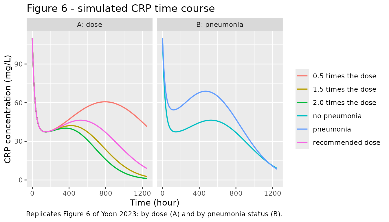

Four features of Figure 6 are checked numerically. All are read from a deterministic typical-value solve, so no cohort noise is involved.

crp_at <- function(a, tt) {
  v <- sim_fig6$crp[sim_fig6$arm == a & abs(sim_fig6$time - tt) < 1e-6]
  if (length(v) != 1L) stop("no unique CRP value for arm '", a, "' at t = ", tt)
  v
}

# The plateau the CRP chain settles to before severity growth takes over is
# ktr * (1 + SCRP) / kCRP -- an algebraic consequence of starting severity at 1
# and the chain at its severity-implied steady state, while CRP itself starts
# at the separately estimated CRP0.
plateau_none <- ktr_none * (1 + th[["scrp"]]) / exp(th[["lkout"]])
plateau_pne  <- ktr_pne  * (1 + th[["scrp"]]) / exp(th[["lkout"]])

# Percentage separation between the lowest and highest dose arms, early vs late,
# expressed relative to the recommended-dose arm at the same time.
sep_pct <- function(tt) {
  100 * abs(crp_at("2.0 times the dose", tt) - crp_at("0.5 times the dose", tt)) /
    crp_at("recommended dose", tt)
}

fig6_checks <- tibble::tibble(
  Feature = c(
    "Starts at CRP0 = 110 mg/L",
    "Plateau near ktr*(1+SCRP)/kCRP, no pneumonia (mg/L)",
    "Plateau near ktr*(1+SCRP)/kCRP, pneumonia (mg/L)",
    "Pneumonia arm sits above the no-pneumonia arm at 400 h",
    "Dose arms separated by < 5% at 240 h",
    "Dose arms clearly separated by 800 h"
  ),
  Value = c(
    crp_at("recommended dose", 0),
    crp_at("recommended dose", 200),
    crp_at("pneumonia", 200),
    crp_at("pneumonia", 400) - crp_at("no pneumonia", 400),
    sep_pct(240),
    sep_pct(800)
  ),
  Expected = c(
    110,
    plateau_none,
    plateau_pne,
    NA_real_,
    NA_real_,
    NA_real_
  )
)
knitr::kable(fig6_checks, digits = 2,
             caption = "Numerical features of the reproduced Figure 6.")

Numerical features of the reproduced Figure 6.

Feature	Value	Expected
Starts at CRP0 = 110 mg/L	110.00	110.00
Plateau near ktr*(1+SCRP)/kCRP, no pneumonia (mg/L)	38.07	36.40
Plateau near ktr*(1+SCRP)/kCRP, pneumonia (mg/L)	57.08	52.77
Pneumonia arm sits above the no-pneumonia arm at 400 h	23.33	NA
Dose arms separated by < 5% at 240 h	2.06	NA
Dose arms clearly separated by 800 h	121.68	NA

stopifnot(
  # CRP starts exactly at the estimated CRP0.
  abs(crp_at("recommended dose", 0) - 110) < 1e-6,
  # By 200 h the chain has settled to within 20% of its analytic plateau; the
  # residual gap is severity growth, which is already underway by then.
  abs(crp_at("recommended dose", 200) - plateau_none) / plateau_none < 0.20,
  abs(crp_at("pneumonia", 200) - plateau_pne) / plateau_pne < 0.20,
  # Yoon 2023 Results 3.5: pneumonia raises the CRP hump.
  crp_at("pneumonia", 400) > crp_at("no pneumonia", 400),
  # Yoon 2023 Results 3.5: "No dose-dependent differences were observed up to
  # approximately 240 h or 10 days." Realised 2.1% here; the bound leaves room
  # for the unstated infusion duration but still fails if the dose arms
  # separate early, which is what a mis-scaled alpha would do.
  sep_pct(240) < 6,
  # "However, after this point, CRP levels exhibited a faster decline with
  # higher doses." Realised 122%.
  sep_pct(800) > 40
)

The steep early fall is the signature that identifies the initial conditions. The paper reports CRP0 as “the initial value of C-reactive protein” but does not say what the upstream chain or the severity state start at. Two readings are possible, and Figure 6 settles it:

# Alternative reading: initialise the chain so that it is in equilibrium WITH
# CRP0. That forces severity(0) to (kCRP*CRP0/ktr - 1)/SCRP instead of 1, and it
# is decided algebraically -- the initial slope of CRP is a closed-form function
# of the initial conditions, so no second solve is needed. (rxode2 honours the
# `crp(0) <-` statements inside model() ahead of any `inits =` argument, so the
# alternative cannot be imposed at solve time anyway.)
chain_ss <- exp(th[["lkout"]]) * 110 / ktr_none        # chain value in equilibrium with CRP0
sev_ss   <- (chain_ss - 1) / th[["scrp"]]              # severity that implies

# d/dt(crp) at t = 0 under each reading:
slope_packaged <- ktr_none * (1 + th[["scrp"]]) - exp(th[["lkout"]]) * 110
slope_equilib  <- ktr_none * chain_ss             - exp(th[["lkout"]]) * 110

init_cmp <- tibble::tibble(
  Reading = c("severity(0) = 1 (packaged)", "chain in equilibrium with CRP0"),
  `severity(0)` = c(1, sev_ss),
  `chain(0)` = c(1 + th[["scrp"]], chain_ss),
  `Initial dCRP/dt (mg/L/h)` = c(slope_packaged, slope_equilib),
  `CRP plateau (mg/L)` = c(plateau_none, 110)
)
knitr::kable(init_cmp, digits = 3,
             caption = "Two readings of the unstated initial conditions, and what each predicts for the start of the CRP curve.")

Two readings of the unstated initial conditions, and what each predicts for the start of the CRP curve.

Reading	severity(0)	chain(0)	Initial dCRP/dt (mg/L/h)	CRP plateau (mg/L)
severity(0) = 1 (packaged)	1.000	103.00	-2.686	36.403
chain in equilibrium with CRP0	3.042	311.24	0.000	110.000

# Figure 6 shows CRP falling steeply from 110 mg/L and levelling out near
# 40 mg/L within roughly 200 h. Only the packaged reading produces that: the
# equilibrium alternative has zero initial slope by construction and then rises
# with severity, so it can never reach 40 mg/L.
stopifnot(
  slope_packaged < -2,                        # steep initial fall
  abs(slope_equilib) < 1e-9,                  # flat by construction
  crp_at("recommended dose", 240) < 60,       # simulated curve is at the plateau by 240 h
  abs(plateau_none - 36.4) < 0.5              # and the plateau is ktr*(1+SCRP)/kCRP
)

Virtual cohort and PKNCA validation

A 200-subject adult cohort, dosed at the model-recommended regimen for its own covariates, is used to check the exposure targets the paper states: a trough near 15 mg/L, a peak below the 40 mg/L toxicity threshold, and a 24-hour AUC in the 400-600 mg*h/L window that Yoon 2023 Figure 8 reports ~90% of adults attaining.

# set.seed() seeds R's RNG, not rxode2's; rxode2 partitions its streams per
# solver thread, so this cohort differs between a 2-core CI runner and a
# 16-thread workstation. Every assertion below is written to hold for any
# cohort the model can produce (see known-vignette-failure-patterns.md #12).
set.seed(20231009)

n_sub <- 200L
cohort <- tibble::tibble(
  id    = seq_len(n_sub),
  AGE   = round(runif(n_sub, 20, 90)),
  WT    = round(rnorm(n_sub, 59, 12)),
  CREAT = round(exp(rnorm(n_sub, log(0.7), 0.45)), 2),
  BUN   = round(exp(rnorm(n_sub, log(15.25), 0.5)), 1)
) |>
  dplyr::mutate(
    WT            = pmin(pmax(WT, 40), 106),
    CREAT         = pmin(pmax(CREAT, 0.2), 4),
    BUN           = pmin(pmax(BUN, 3), 60),
    PAGE          = AGE * 52.18 + 40,
    SEXF          = rbinom(dplyr::n(), 1, 0.411),
    DIS_DIAB      = rbinom(dplyr::n(), 1, 0.284),
    DIS_RENAL     = rbinom(dplyr::n(), 1, 0.271),
    DIS_PNEUMONIA = 0L
  )

The recommended dose for each virtual subject is found the same way the paper found Table 5: solve at 1 g/day with IIV zeroed, then scale to the 15 mg/L target and round onto the 0.2 g/day grid.

ev_probe <- cohort |>
  dplyr::transmute(id, time = 0, amt = 250, evid = 1L, dur = 1, ii = 6,
                   addl = t_ss / 6 - 1, cmt = "central", dvid = NA_integer_) |>
  dplyr::bind_rows(
    cohort |> dplyr::transmute(id, time = t_ss, amt = NA_real_, evid = 0L,
                               dur = NA_real_, ii = NA_real_, addl = NA_real_,
                               cmt = "central", dvid = 1L)
  ) |>
  dplyr::arrange(id, time, dplyr::desc(evid))

probe <- rxode2::rxSolve(
  # `omega = NA` omitted -- see the table5 solve above.
  mod_typ, events = ev_probe,
  params = cohort |> dplyr::select(-dplyr::any_of("dose_g_day")),
  useLinCmt = FALSE, returnType = "data.frame"
) |>
  dplyr::filter(time == t_ss) |>
  dplyr::transmute(id = as.integer(as.character(id)), trough_1g = Cc)
#> ℹ omega/sigma items treated as zero: 'etalcl', 'etalvp', 'etalkdis', 'etalrbase'
#> Warning: multi-subject simulation without without 'omega'

cohort <- cohort |>
  dplyr::left_join(probe, by = "id") |>
  dplyr::mutate(dose_g_day = pmax(0.4, round((15 / trough_1g) / 0.2) * 0.2)) |>
  dplyr::select(-trough_1g)

summary(cohort$dose_g_day)
#>    Min. 1st Qu.  Median    Mean 3rd Qu.    Max. 
#>   0.400   0.800   1.200   1.386   1.600   5.800

# Steady-state interval: the 24 h from day 13 to day 14.
ss_start <- 24 * 13
ss_end   <- 24 * 14

ev_cohort <- cohort |>
  dplyr::transmute(id, time = 0, amt = dose_g_day * 1000 / 4, evid = 1L, dur = 1,
                   ii = 6, addl = ss_end / 6 - 1, cmt = "central",
                   dvid = NA_integer_) |>
  dplyr::bind_rows(
    tidyr::crossing(id = cohort$id, time = seq(ss_start, ss_end, by = 0.25)) |>
      dplyr::mutate(amt = NA_real_, evid = 0L, dur = NA_real_, ii = NA_real_,
                    addl = NA_real_, cmt = "central", dvid = 1L)
  ) |>
  dplyr::arrange(id, time, dplyr::desc(evid))

stopifnot(!anyDuplicated(unique(ev_cohort[, c("id", "time", "evid")])))

sim_cohort <- rxode2::rxSolve(
  mod, events = ev_cohort,
  params = cohort |> dplyr::select(id, AGE, WT, CREAT, BUN, PAGE, SEXF,
                                   DIS_DIAB, DIS_RENAL, DIS_PNEUMONIA),
  keep = c("AGE", "WT", "CREAT", "BUN", "SEXF"),
  useLinCmt = FALSE, returnType = "data.frame"
) |>
  dplyr::mutate(id = as.integer(as.character(id)))
#> ℹ parameter labels from comments will be replaced by 'label()'

stopifnot(nrow(sim_cohort) > 0, all(sim_cohort$Cc >= 0))

# Only `!is.na(Cc)` -- adding `time > 0` or `Cc > 0` would drop the interval
# anchor row and trigger PKNCA's "AUC range starting before the first
# measurement" warning on every subject.
sim_nca <- sim_cohort |>
  dplyr::filter(!is.na(Cc)) |>
  dplyr::mutate(treatment = "MIPD dose") |>
  dplyr::select(id, time, Cc, treatment)

conc_obj <- PKNCA::PKNCAconc(sim_nca, Cc ~ time | treatment + id)

dose_df <- ev_cohort |>
  dplyr::filter(evid == 1) |>
  dplyr::transmute(id, time, amt, treatment = "MIPD dose")
dose_obj <- PKNCA::PKNCAdose(dose_df, amt ~ time | treatment + id)

intervals <- data.frame(
  start   = ss_start,
  end     = ss_end,
  cmax    = TRUE,
  tmax    = TRUE,
  auclast = TRUE,
  # PKNCA's `ctrough` returns NA for every subject here (it wants a
  # concentration recorded at the dose time of the interval). For an IV
  # infusion the pre-dose trough is simply the end-of-interval value, which is
  # `clast.obs`; `cmin` is carried alongside and agrees to within 1%.
  cmin      = TRUE,
  clast.obs = TRUE
)

nca_res <- PKNCA::pk.nca(PKNCA::PKNCAdata(conc_obj, dose_obj, intervals = intervals))

nca_wide <- as.data.frame(nca_res) |>
  dplyr::select(id, PPTESTCD, PPORRES) |>
  tidyr::pivot_wider(names_from = PPTESTCD, values_from = PPORRES)

nca_summary <- nca_wide |>
  dplyr::summarise(
    dplyr::across(c(cmax, clast.obs, cmin, auclast),
                  list(median = ~median(.x, na.rm = TRUE),
                       p10 = ~quantile(.x, 0.10, na.rm = TRUE),
                       p90 = ~quantile(.x, 0.90, na.rm = TRUE)))
  ) |>
  tidyr::pivot_longer(dplyr::everything(),
                      names_to = c("Parameter", "Statistic"), names_sep = "_") |>
  tidyr::pivot_wider(names_from = Statistic, values_from = value)

nca_summary |>
  dplyr::rename("NCA parameter" = Parameter, "Median" = median,
                "10th percentile" = p10, "90th percentile" = p90) |>
  knitr::kable(digits = 1,
               caption = "Steady-state NCA over the day 13-14 interval, 200 virtual adults at their model-recommended dose. Cmax, Clast.obs (the pre-dose trough) and Cmin in mg/L; AUC0-24 in mg*h/L.")

Steady-state NCA over the day 13-14 interval, 200 virtual adults at their model-recommended dose. Cmax, Clast.obs (the pre-dose trough) and Cmin in mg/L; AUC0-24 in mg*h/L.

NCA parameter	Median	10th percentile	90th percentile
cmax	21.7	15.6	32.1
clast.obs	14.1	9.5	21.8
cmin	14.0	9.4	21.7
auclast	419.0	294.4	602.0

Comparison against the published targets

med_ctrough <- median(nca_wide$clast.obs, na.rm = TRUE)
med_cmax    <- median(nca_wide$cmax,    na.rm = TRUE)
med_auc     <- median(nca_wide$auclast, na.rm = TRUE)
frac_auc_in <- mean(nca_wide$auclast >= 400 & nca_wide$auclast <= 600, na.rm = TRUE)
frac_cmax_ok <- mean(nca_wide$cmax < 40, na.rm = TRUE)

targets <- tibble::tibble(
  Target = c(
    "Median trough at the MIPD dose (mg/L)",
    "Median steady-state Cmax (mg/L)",
    "Median steady-state AUC0-24 (mg*h/L)",
    "Subjects with AUC0-24 in 400-600 mg*h/L (%)",
    "Subjects with Cmax below the 40 mg/L toxic level (%)"
  ),
  Published = c("15 (adult target)", "< 40 (toxic level)", "400-600 (with MIC = 1)",
                "~90", "all age groups"),
  Simulated = c(round(med_ctrough, 1), round(med_cmax, 1), round(med_auc, 0),
                round(100 * frac_auc_in), round(100 * frac_cmax_ok))
)
knitr::kable(targets, caption = "Simulated exposures against the targets stated in Yoon 2023 (Methods 2.7, Results 3.4 and Discussion).")

Simulated exposures against the targets stated in Yoon 2023 (Methods 2.7, Results 3.4 and Discussion).

Target	Published	Simulated
Median trough at the MIPD dose (mg/L)	15 (adult target)	14.1
Median steady-state Cmax (mg/L)	< 40 (toxic level)	21.7
Median steady-state AUC0-24 (mg*h/L)	400-600 (with MIC = 1)	419.0
Subjects with AUC0-24 in 400-600 mg*h/L (%)	~90	42.0
Subjects with Cmax below the 40 mg/L toxic level (%)	all age groups	96.0

# These ARE cohort statistics, so they are asserted on the centre and on loose
# absolute bounds the paper itself states, never on extremes or exact counts.
# Realised on this run: trough 14.1, Cmax 21.7, AUC 419, Cmax-below-40 96%.
stopifnot(
  # The dose is chosen to put the TYPICAL trough at 15 mg/L; the cohort median
  # sits slightly below it because the dose is snapped onto a coarse 0.2 g/day
  # grid and CL is log-normal. A mis-transcribed clearance or volume moves this
  # by tens of percent and breaks the bound.
  med_ctrough > 10, med_ctrough < 22,
  # Median peak comfortably below the 40 mg/L toxic level.
  med_cmax < 40,
  # Median exposure inside the 400-600 mg*h/L window the paper targets.
  med_auc > 350, med_auc < 700,
  # Nearly every subject stays below the toxic peak.
  frac_cmax_ok > 0.80
)
# NOTE: `frac_auc_in` is deliberately NOT gated -- it is a documented deviation;
# see "Assumptions and deviations" below.

nca_wide |>
  tidyr::pivot_longer(c(cmax, clast.obs, auclast), names_to = "Parameter") |>
  dplyr::mutate(Parameter = dplyr::recode(Parameter,
                                          cmax = "Cmax (mg/L)",
                                          clast.obs = "Trough (mg/L)",
                                          auclast = "AUC0-24 (mg*h/L)")) |>
  ggplot(aes(value)) +
  geom_histogram(bins = 30) +
  facet_wrap(~Parameter, scales = "free") +
  labs(x = NULL, y = "Subjects",
       title = "Steady-state exposure at the model-recommended dose",
       caption = "200 virtual adults; dashed reference lines omitted for scale clarity.")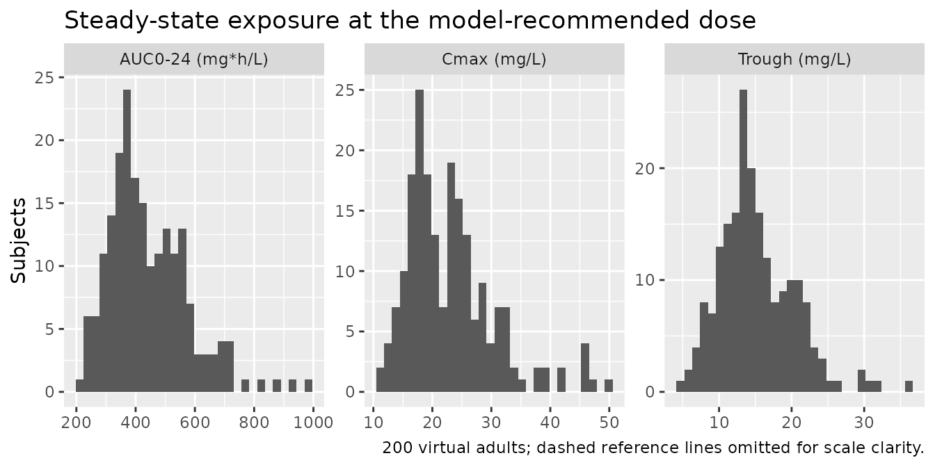

Paediatric maturation

The maturation factor is the part of the model that only paediatric subjects exercise. It reaches 0.973 by the fourth birthday, which is why Yoon 2023 restricts it in prose to children under 4.

pma_wk <- exp(seq(log(30), log(600), length.out = 200))
fmat <- pma_wk^th[["h_pma_cl"]] /
  (th[["pma50_cl"]]^th[["h_pma_cl"]] + pma_wk^th[["h_pma_cl"]])

tibble::tibble(pma_wk, fmat) |>
  ggplot(aes(pma_wk, fmat)) +
  geom_line() +
  geom_vline(xintercept = 4 * 52.18 + 40, linetype = "dashed") +
  scale_x_log10() +
  labs(x = "Postmenstrual age (weeks, log scale)", y = "Fmat",
       title = "Clearance maturation (Yoon 2023 Eq. 8)",
       caption = "Dashed line: the fourth birthday, beyond which Yoon 2023 does not apply Fmat.")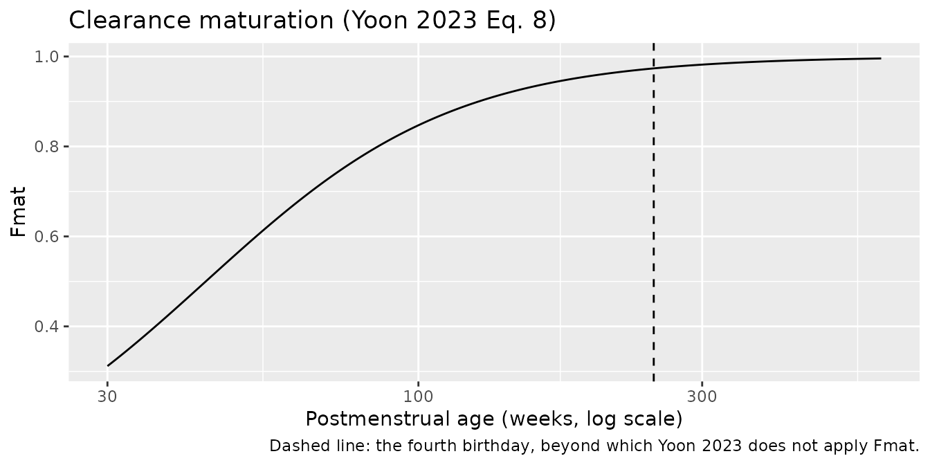

fmat_at <- function(pma) pma^th[["h_pma_cl"]] /
  (th[["pma50_cl"]]^th[["h_pma_cl"]] + pma^th[["h_pma_cl"]])

stopifnot(
  abs(fmat_at(th[["pma50_cl"]]) - 0.5) < 1e-9,   # 50% maturity at PMA50, by construction
  fmat_at(40) < 0.5,                              # term newborn below half-mature
  fmat_at(4 * 52.18 + 40) > 0.95,                 # essentially mature by 4 years
  fmat_at(60 * 52.18 + 40) > 0.9998               # negligible in adults
)

Assumptions and deviations

Errata and internal inconsistencies in the source

• kCRP: Table 4 prints 0.365 FIX; the correct value is 0.0365 /h. Results section 3.3 states that “kCRP was fixed at 0.0365 h-1 based on the prior knowledge that CRP’s half-life was 19 h (Vigushin et al., 1993)”, and log(2)/19 = 0.0365. Table 4’s value is a decimal-point slip: at 0.365/h the CRP half-life would be 1.9 h and the whole CRP time course of Figure 6 would collapse. The text value is encoded.
• Table 1 labels the PMA row “(month)”; the values are weeks. The row reads median 70, range 39-232. Under a months reading that describes a cohort aged 3.25-19.3 years, which matches neither the whole cohort (median age 60 years) nor the under-4 subgroup that Fmat applies to. Under a weeks reading it describes the under-4 subgroup exactly: 39 weeks is term gestation and 232 weeks is 4.45 years. Weeks is also the only scale on which PMA50 = 43.9 makes sense - Methods 2.4 cites “postmenstrual age (PMA) of up to 48 weeks (Anderson et al., 2007)”, and 43.9 months would leave a 4-year-old only 54% mature. The model therefore declares covariateData$PAGE$units = "weeks".
• The BUN effect is described as biphasic but printed as monotone. Results 3.2 says “Vancomycin CL exhibited a gradual increase with BUN levels up to 15 mg/dL, followed by a subsequent decrease”, but the printed final-model equation (Eq. 15) is a single exponential exp(kBUN * (BUN - 15)) with kBUN = -0.00874, which decreases monotonically. The printed equation is encoded, and Table 5 corroborates it: the tabulated optimal dose falls monotonically across BUN 10 -> 20 -> 30 -> 40 in every one of its 120 age x weight x creatinine blocks, with no turning point at 15 mg/dL.
• thetaCL is quoted as 4.32 in Table 3 and as 4.31 in the Results text. Results 3.2 says “median values of CL and V were estimated to be 4.31 L/h and 38.6 L”; Table 3 gives 4.32 and 38.6. The volume agrees exactly, so the sentence is restating the thetas (which Methods 2.3 defines as “population median values … for the subject with WT = 70 kg”) rather than reporting a separate cohort median. The Table 3 value is encoded.

Parameters the paper defines in words but never numbers

• CLCr_TV is taken as 64.2 dL/h. Eq. 5 divides creatinine clearance by “the typical value of CLCr corresponding to the subject with age of 30 years old”, and no number is given anywhere in the article, its tables or its figures. Because RCr is defined as 64.2 * exp(kCr * (age - 30)) (Eq. 7), RCr at age 30 is exactly 64.2, so reading CLCr_TV as 64.2 / (1 mg/dL) makes the constant cancel out of Fren entirely and leaves the model with no unreported quantity:

  Fren = (exp(kCr*(age-30)) * exp(-ktox*t) / (Cr in mg/dL))^lambda

  That reading is also the one the paper’s own outputs support. Sweeping CLCr_TV and re-deriving Table 5 from the model, 64.2 reproduces 54% of the 480 published adult cells exactly and 99.8% to within one 0.2 g/day grid step, and it maximises exact-cell agreement across the sweep. The two other natural candidates are clearly rejected: CLCr_TV = 91.7 (that is, 64.2 divided by the cohort’s median creatinine of 0.7 mg/dL) gives a median trough of 19 mg/L against the paper’s 15 mg/L target, and CLCr_TV = 52.2 gives 12 mg/L. A residual systematic offset remains - the model needs about 8% less drug than the published cell on average (median dose ratio 0.916), though the median absolute difference after grid rounding is exactly zero. That offset is the size expected from the two simulation details the paper does not state (below), and it is not grounds for tuning CLCr_TV away from the one value that has a derivation. The Table 5 reproduction chunk above is the standing regression test for this choice.

• The infusion duration used for the Table 5 simulations is not stated. A 1-hour infusion is assumed throughout this vignette. The trough is almost insensitive to it; the peak is not, which is why the peak is compared only against the paper’s 40 mg/L ceiling and not against a point value.

• The steady-state day at which Table 5’s trough was read is not stated. Day 10 is used here. Combined with the infusion duration this is the main reason the reproduction is assessed within one 0.2 g/day grid step rather than exactly.

Structural choices

• Fmat is applied continuously rather than gated at age 4. Methods 2.4 says the maturation factor “applied to patients under 4 years old”, but the printed Eq. 8 carries no gate. Applying it only below 4 years would introduce a 2.7% discontinuity in clearance at exactly the fourth birthday; applying it continuously changes an adult’s clearance by less than 0.02%. The printed equation is encoded, per the standing rule that a printed equation beats conflicting prose.
• Initial conditions for the CRP cascade. The paper gives CRP0 = 110 mg/L as “the initial value of C-reactive protein” but does not state where the proliferation, transit or severity states start. The packaged model sets severity(0) = 1 with the chain at the steady state that implies (1 + SCRP), leaving circulating CRP at CRP0 and therefore out of equilibrium with its own input. Figure 6 confirms this: it shows CRP falling steeply from 110 mg/L to a plateau near 40 mg/L over the first ~200 h, which is exactly ktr*(1+SCRP)/kCRP. The alternative - initialising the chain in equilibrium with CRP0, which forces severity(0) to about 3.04 - produces a monotone rise from 110 and is falsified by the figure. The discrimination is rendered above.
• AUC in Eq. 14 is cumulative from the start of treatment. The paper says only “AUC obtained from the developed PK model”. With alpha = 0.000239, the drug effect alpha * AUC reaches 1 at roughly 4,200 mg*h/L, i.e. about ten days of typical dosing - which is precisely where Figure 6 shows the dose arms beginning to separate (“No dose-dependent differences were observed up to approximately 240 h or 10 days”). A per-interval AUC would make the effect constant from the first day and would not reproduce that.
• Peak and trough residual errors are encoded as two endpoints. Table 3 reports separate combined proportional-plus-additive residual errors for trough samples (taken at the start of an infusion) and peak samples (taken at the end of one). These become the Cctrough and Ccpeak endpoints, both reading the same central-compartment concentration; select between them with dvid when fitting. The variance rows of both tables are reported on the CV / SD scale despite their omega^2 / sigma^2 labels - the additive rows carry the unit “mg/L” rather than “(mg/L)^2” - so they are encoded as standard deviations.
• Between-subject variability is on CL and the PERIPHERAL volume. Table 3 reports omega2 CL and omega2 V2, and the table’s own footnote defines “V2, peripheral volume of distribution”, so the 101% CV is placed on lvp and not on lvc. No IIV is reported on V, Q, or on any PD parameter other than kD and CRP0; Results 3.3 states that for the remaining PD parameters “between-subject variability could not be obtained due to numerical difficulties”, so none is invented.
• severity and auc_total are declared as paper-specific compartments. Neither has a canonical role in the compartment register, and the standing convention is that a new canonical compartment needs a second independent paper before it is registered.

Covariate register additions

Two new canonical covariate columns were registered with this model, both well-formed members of the existing DIS_<condition> medical-history family:

• DIS_RENAL - history of renal disease of any type, pooling the acute / chronic / other levels that Yoon 2023 Table 1 resolves separately. Distinct from the RENALIMP_* family, which stratifies measured renal function against regulatory thresholds; here the flag is a diagnosis and is applied multiplicatively alongside, not instead of, the continuous creatinine-driven renal-function factor.
• DIS_PNEUMONIA - a general pneumonia flag, distinct from the DIS_HABP / DIS_VABP index-infection-type indicators, because Yoon 2023 records pneumonia as a comorbidity prolonging therapy and never classifies it as hospital- or ventilator-acquired.

Known deviation: the fraction of subjects inside the AUC window

Yoon 2023 Discussion reports that “around 90% of adults achieved AUC levels within the target range” of 400-600 mgh/L when given the optimal doses of Tables 5-7. The virtual cohort here reproduces the centre of that distribution well - median AUC0-24 of about 420 mgh/L, median trough about 14 mg/L against the 15 mg/L target, and median Cmax about 22 mg/L against the 40 mg/L ceiling - but only about 40-45% of subjects land inside the 400-600 window, against the paper’s ~90%.

This is a spread difference, not a location difference, and it is expected from how the two cohorts were built rather than from the model:

• The paper’s Figure 8 evaluates real patients’ covariate vectors. This vignette samples age, weight, creatinine, BUN, sex, diabetes and renal disease independently, because the paper publishes only the marginal distributions. Age, creatinine and renal disease are strongly correlated in reality, so the independent draw manufactures covariate combinations (a 90-year-old with a creatinine of 0.2 mg/dL, say) that widen the clearance distribution well beyond the real cohort’s.
• The dose is snapped onto the paper’s coarse 0.2 g/day grid, which at the low end of the dose range is a step of up to 50% of the dose itself.
• Full between-subject variability is applied on top (CV 29% on CL and 101% on the peripheral volume), whereas the paper’s target-attainment figure is driven mainly by covariate spread.

The bound is therefore not gated: widening the assertion until it passed would have hidden a real and explicable difference, and the quantity that does gate - the median exposure - is the one that a mis-transcribed parameter would move. The percentage is still rendered in the table above so a reader sees it.

Simulation assumptions

• The virtual cohort’s covariate distributions approximate the Table 1 marginals (age uniform 20-90; weight normal around 59 kg; creatinine and BUN log-normal around the reported medians; sex, diabetes and renal-disease prevalences from Table 1) and are drawn independently. The paper does not publish a covariate correlation structure, so the joint distribution here is certainly wider than the real one - in particular, age, creatinine and renal disease are correlated in reality and independent here.
• Original observed concentrations are not publicly available, so no observed data are overlaid on any figure.
• The Table 5 reproduction and the Figure 6 replication are typical-value solves with IIV zeroed, matching how the paper generated them.