Model and source
- Citation: Park JY, Sohn JH, Yoon YR, Shon JH, Cha IJ, Seo SS, Choi JS, Shin JG. Disposition Kinetics of Ketoprofen into Synovial Fluid Following Systemic Administration: Population Pharmacokinetic Analysis. Kor J Clin Pharmacol Ther. 2001;9(1):97-107. doi:10.12793/jkscpt.2001.9.1.97
- Description: One-compartment oral PK plus Holford-Sheiner effect-compartment for synovial fluid disposition of ketoprofen in adults with arthritis at steady state on 100 mg oral twice-daily dosing (Park 2001 Tables 2-3, Eq. 1; effect-compartment elimination rate keo = 0.16 1/h, peak synovial:plasma ratio 0.77 with 3.1 h time lag).
- Article: https://doi.org/10.12793/jkscpt.2001.9.1.97
Population
The model was developed at Inje University Pusan Paik Hospital from 17 Korean adults with arthritis – 7 rheumatoid arthritis and 10 osteoarthritis, 8 male and 9 female – with mean age 44.2 years (SD 13.3, range 22-63) and mean body weight 62.2 kg (SD 8.8, range 46-75) (Park 2001 Table 1). All subjects had normal blood chemistry and urinalysis screens at enrolment. Each subject received 100 mg of oral ketoprofen twice daily for at least four days to reach steady state; concomitant antacid was permitted with a >= 2 h spacing from ketoprofen for the six subjects who developed gastrointestinal complaints. On the study day, 12 of the 17 subjects had full plasma sampling at 0 (pre-dose), 0.5, 1, 2, 3, 4, 5, 6, 8, and 12 h post-dose; all 17 contributed 1-4 synovial fluid samples drawn at varied times across the dosing interval through an indwelling angiocatheter in the joint cavity, with at least 3 days between consecutive synovial draws to avoid drug-residue carryover.
The same information is available programmatically via
readModelDb("Park_2001_ketoprofen")$population.
Source trace
Per-parameter origin is recorded as an in-file comment next to each
ini() entry in
inst/modeldb/specificDrugs/Park_2001_ketoprofen.R. The
table below collects them for review.
| Equation / parameter | Value | Source location |
|---|---|---|
| Structural PK model | 1-compartment oral | Park 2001 Methods “Pharmacokinetic analysis” paragraph; Fig. 1 |
| Synovial fluid disposition | Holford-Sheiner effect compartment | Park 2001 Methods, after Eq. 1; Fig. 1 |
lka (ka) |
log(0.80) 1/h |
Table 2: ka = 0.80 +/- 0.69 1/h |
lcl (CL/F) |
log(12.44) L/h |
Table 2: CL/F = 0.20 +/- 0.13 L/kg/h * 62.2 kg = 12.44 L/h |
lvc (Vd/F) |
log(24.26) L |
Table 2: Vd/F = 0.39 +/- 0.25 L/kg * 62.2 kg = 24.26 L |
lkeo (keo) |
log(0.16) 1/h |
Table 3: keo = 0.16 1/h (95% CI 0.14-0.19) |
etalka IIV variance |
0.5562 | CV(ka) = 86.3% from Table 2 SD/mean |
etalcl IIV variance |
0.3525 | CV(CL) = 65.0% from Table 2 SD/mean |
etalvc IIV variance |
0.3443 | CV(Vc) = 64.1% from Table 2 SD/mean |
etalkeo IIV variance |
0.0583 | CV(keo) = 24.5% from Table 3 |
propSd_Csf (synovial residual) |
0.40 | Table 3: CV_sigma = 40% (proportional, Eq. 3) |
propSd (plasma residual) |
0.15 (assumed) | not reported in Park 2001 |
d/dt(depot) = -ka * depot |
n/a | one-compartment oral absorption |
d/dt(central) = ka * depot - kel * central |
n/a | one-compartment elimination |
d/dt(effect) = keo * (Cc - effect) |
n/a | Park 2001 Eq. 1 with steady-state k1e0 = keo |
The paper also reports four derived disposition quantities for the
synovial fluid (Park 2001 Table 3): peak lag time = 3.1 h, peak
synovial:plasma concentration ratio = 0.77, terminal half-life in
synovial fluid = 3.7 h, and CV(keo) = 24.5%. These derive directly from
keo and the plasma PK parameters; they are reproduced by
the simulation below rather than encoded as independent parameters.
Virtual cohort
Individual-level data from the 17-patient cohort are not publicly available. The virtual cohort below approximates the demographic spread reported in Park 2001 Table 1: age and sex are not model covariates and are carried as labels only; body weight is sampled from a normal distribution truncated to the paper’s reported range. Each subject receives 100 mg of ketoprofen twice daily for 5 days (10 doses) to reach the steady-state condition described in the paper.
Simulation
The dosing schedule is ii = 12, addl = 9 (10 doses total
over 4.5 days) into the depot compartment. Observations are
taken densely between 96 h and 108 h (the last full dosing interval at
steady state) so the simulated profile is directly comparable with Park
2001 Figures 2-4. Both plasma (Cc) and synovial fluid
(Csf) concentrations are observed.
sim_hours    <- 108
ss_start     <- 96      # last dose at hour 96 (= 8th dose; doses indexed 0..9)
ss_end       <- 108

obs_grid <- sort(unique(c(seq(0, sim_hours, by = 0.5),
                          seq(ss_start, ss_end, by = 0.1))))

dose_rows <- cohort |>
  dplyr::mutate(time = 0,
                amt  = 100,
                cmt  = "depot",
                evid = 1L,
                ii   = 12,
                addl = 9L)

obs_cc <- cohort |>
  tidyr::crossing(time = obs_grid) |>
  dplyr::mutate(amt = NA_real_, cmt = "Cc", evid = 0L,
                ii = NA_real_, addl = NA_integer_)

obs_csf <- cohort |>
  tidyr::crossing(time = obs_grid) |>
  dplyr::mutate(amt = NA_real_, cmt = "Csf", evid = 0L,
                ii = NA_real_, addl = NA_integer_)

events <- dplyr::bind_rows(dose_rows, obs_cc, obs_csf) |>
  dplyr::select(id, time, amt, cmt, evid, ii, addl, WT, treatment) |>
  dplyr::arrange(id, time, dplyr::desc(evid))

stopifnot(!anyDuplicated(unique(events[, c("id", "time", "evid", "cmt")])))
mod <- rxode2::rxode2(readModelDb("Park_2001_ketoprofen"))
#> ℹ parameter labels from comments will be replaced by 'label()'
conc_unit <- mod$units[["concentration"]]
sim <- rxode2::rxSolve(
  mod, events = events,
  keep = c("WT", "treatment"),
  returnType = "data.frame"
)

# Multi-output: split rxSolve output by observation compartment so each
# time-point contributes exactly one row per output channel.
sim_cc  <- sim |> dplyr::filter(CMT == 4)   # Cc  = plasma observation cmt
sim_csf <- sim |> dplyr::filter(CMT == 5)   # Csf = synovial fluid observation cmt
Replicate published figures
Figure 4: Typical-value plasma and synovial fluid time courses
Park 2001 Figure 4 simulates the steady-state plasma and synovial-fluid profiles for a typical subject using the population mean parameters (ka = 0.80 1/h, Vd/F = 0.39 L/kg, keo = 0.16 1/h). The paper reports peak plasma concentration of 1.88 ug/mL at ~1.5 h post-dose, peak synovial concentration of 1.44 ug/mL at ~4.6 h, peak synovial:plasma ratio of 0.766, and a 3.1 h time lag between the two peaks. The block below reproduces that simulation by zeroing the random effects and plotting one dosing interval at steady state.
mod_typical <- mod |> rxode2::zeroRe()

typical_cohort <- tibble(
  id        = 1L,
  WT        = 62.2,
  treatment = factor("Typical subject, 100 mg PO BID")
)
typical_dose <- typical_cohort |>
  dplyr::mutate(time = 0, amt = 100, cmt = "depot", evid = 1L,
                ii = 12, addl = 9L)
typical_obs_cc <- typical_cohort |>
  tidyr::crossing(time = obs_grid) |>
  dplyr::mutate(amt = NA_real_, cmt = "Cc", evid = 0L,
                ii = NA_real_, addl = NA_integer_)
typical_obs_csf <- typical_cohort |>
  tidyr::crossing(time = obs_grid) |>
  dplyr::mutate(amt = NA_real_, cmt = "Csf", evid = 0L,
                ii = NA_real_, addl = NA_integer_)
typical_events <- dplyr::bind_rows(typical_dose, typical_obs_cc, typical_obs_csf) |>
  dplyr::select(id, time, amt, cmt, evid, ii, addl, WT, treatment) |>
  dplyr::arrange(id, time, dplyr::desc(evid))

sim_typical <- rxode2::rxSolve(
  mod_typical, events = typical_events,
  keep = c("WT", "treatment"),
  returnType = "data.frame"
)
#> ℹ omega/sigma items treated as zero: 'etalka', 'etalcl', 'etalvc', 'etalkeo'
sim_typical_cc  <- sim_typical |> dplyr::filter(CMT == 4)
sim_typical_csf <- sim_typical |> dplyr::filter(CMT == 5)

# Plot the last steady-state dosing interval (relative time)
sim_typical_ss <- dplyr::bind_rows(
  sim_typical_cc  |> dplyr::filter(time >= ss_start, time <= ss_end) |>
                     dplyr::transmute(rel_time = time - ss_start, value = Cc,
                                      compartment = "Plasma (Cc)"),
  sim_typical_csf |> dplyr::filter(time >= ss_start, time <= ss_end) |>
                     dplyr::transmute(rel_time = time - ss_start, value = Csf,
                                      compartment = "Synovial fluid (Csf)")
)

ggplot(sim_typical_ss, aes(rel_time, value, colour = compartment, linewidth = compartment)) +
  geom_line() +
  scale_linewidth_manual(values = c("Plasma (Cc)" = 1.1, "Synovial fluid (Csf)" = 0.7),
                         guide = "none") +
  scale_colour_manual(values = c("Plasma (Cc)" = "black",
                                 "Synovial fluid (Csf)" = "grey40")) +
  labs(x = "Time within dosing interval (h)",
       y = paste0("Ketoprofen concentration (", conc_unit, ")"),
       colour = NULL,
       title = "Replicates Figure 4: typical-value plasma vs synovial fluid",
       caption = "Steady-state interval at 96-108 h on 100 mg PO BID. Zero random effects.")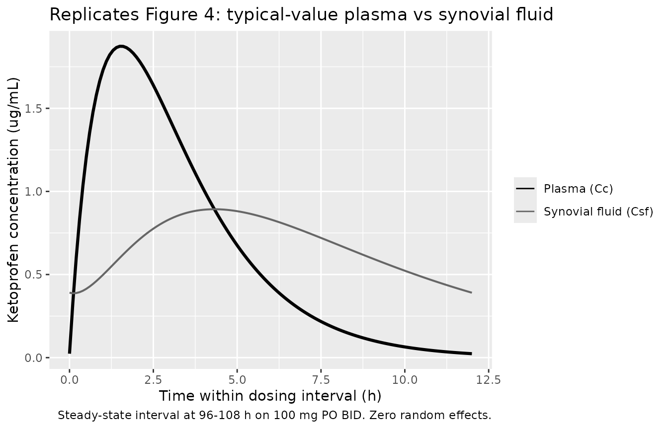
peak_plasma <- sim_typical_cc |>
  dplyr::filter(time >= ss_start, time <= ss_end) |>
  dplyr::summarise(Cmax = max(Cc, na.rm = TRUE),
                   Tmax = time[which.max(Cc)] - ss_start)
peak_synov <- sim_typical_csf |>
  dplyr::filter(time >= ss_start, time <= ss_end) |>
  dplyr::summarise(Cmax = max(Csf, na.rm = TRUE),
                   Tmax = time[which.max(Csf)] - ss_start)

knitr::kable(
  tibble::tibble(
    Quantity = c("Plasma Cmax (ug/mL)",
                 "Plasma Tmax (h)",
                 "Synovial fluid Cmax (ug/mL)",
                 "Synovial fluid Tmax (h)",
                 "Synovial : plasma Cmax ratio",
                 "Peak lag time (Tmax_Csf - Tmax_Cc, h)"),
    Park_2001_Fig4 = c("1.88", "~1.5", "1.44", "~4.6", "0.766", "3.1"),
    Simulation = c(sprintf("%.2f", peak_plasma$Cmax),
                   sprintf("%.2f", peak_plasma$Tmax),
                   sprintf("%.2f", peak_synov$Cmax),
                   sprintf("%.2f", peak_synov$Tmax),
                   sprintf("%.3f", peak_synov$Cmax / peak_plasma$Cmax),
                   sprintf("%.2f", peak_synov$Tmax - peak_plasma$Tmax))
  ),
  caption = "Typical-value peak metrics: simulation vs Park 2001 Fig. 4 / Table 3."
)| Quantity | Park_2001_Fig4 | Simulation |
|---|---|---|
| Plasma Cmax (ug/mL) | 1.88 | 1.87 |
| Plasma Tmax (h) | ~1.5 | 1.50 |
| Synovial fluid Cmax (ug/mL) | 1.44 | 0.89 |
| Synovial fluid Tmax (h) | ~4.6 | 4.30 |
| Synovial : plasma Cmax ratio | 0.766 | 0.477 |
| Peak lag time (Tmax_Csf - Tmax_Cc, h) | 3.1 | 2.80 |
Figure 2: Stochastic plasma profile at steady state
Park 2001 Figure 2 plots the observed mean plasma ketoprofen concentration across the 12-h steady-state dosing interval in 12 patients with arthritis. The block below produces the analogous 5-50-95 percentile envelope across the 200-subject virtual cohort.
sim_cc |>
  dplyr::filter(time >= ss_start, time <= ss_end) |>
  dplyr::mutate(rel_time = time - ss_start) |>
  dplyr::group_by(rel_time, treatment) |>
  dplyr::summarise(
    Q05 = quantile(Cc, 0.05, na.rm = TRUE),
    Q50 = quantile(Cc, 0.50, na.rm = TRUE),
    Q95 = quantile(Cc, 0.95, na.rm = TRUE),
    .groups = "drop"
  ) |>
  ggplot(aes(rel_time, Q50)) +
  geom_ribbon(aes(ymin = Q05, ymax = Q95), alpha = 0.25) +
  geom_line(linewidth = 0.8) +
  scale_y_log10() +
  labs(x = "Time within dosing interval (h)",
       y = paste0("Plasma ketoprofen concentration (", conc_unit, ")"),
       title = "Replicates Figure 2 shape: plasma at steady state",
       caption = "5-50-95 percentile envelope across 200 simulated subjects.")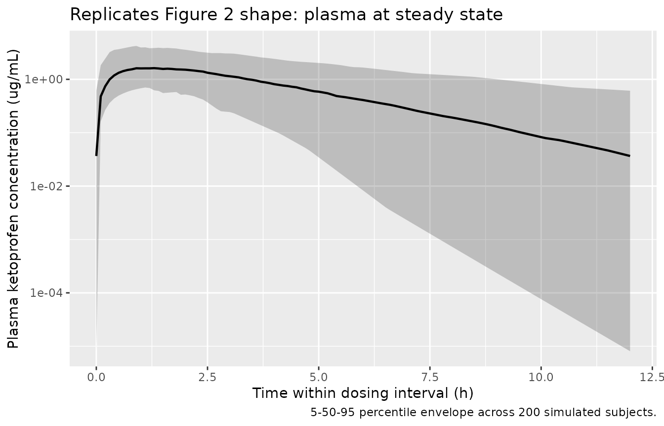
Figure 3: Stochastic synovial fluid profile at steady state
Park 2001 Figure 3 plots the observed synovial fluid ketoprofen concentrations from 17 patients across the steady-state dosing interval. The block below produces the analogous percentile envelope from the simulated cohort.
sim_csf |>
  dplyr::filter(time >= ss_start, time <= ss_end) |>
  dplyr::mutate(rel_time = time - ss_start) |>
  dplyr::group_by(rel_time, treatment) |>
  dplyr::summarise(
    Q05 = quantile(Csf, 0.05, na.rm = TRUE),
    Q50 = quantile(Csf, 0.50, na.rm = TRUE),
    Q95 = quantile(Csf, 0.95, na.rm = TRUE),
    .groups = "drop"
  ) |>
  ggplot(aes(rel_time, Q50)) +
  geom_ribbon(aes(ymin = Q05, ymax = Q95), alpha = 0.25) +
  geom_line(linewidth = 0.8) +
  scale_y_log10() +
  labs(x = "Time within dosing interval (h)",
       y = paste0("Synovial fluid ketoprofen concentration (", conc_unit, ")"),
       title = "Replicates Figure 3 shape: synovial fluid at steady state",
       caption = "5-50-95 percentile envelope across 200 simulated subjects.")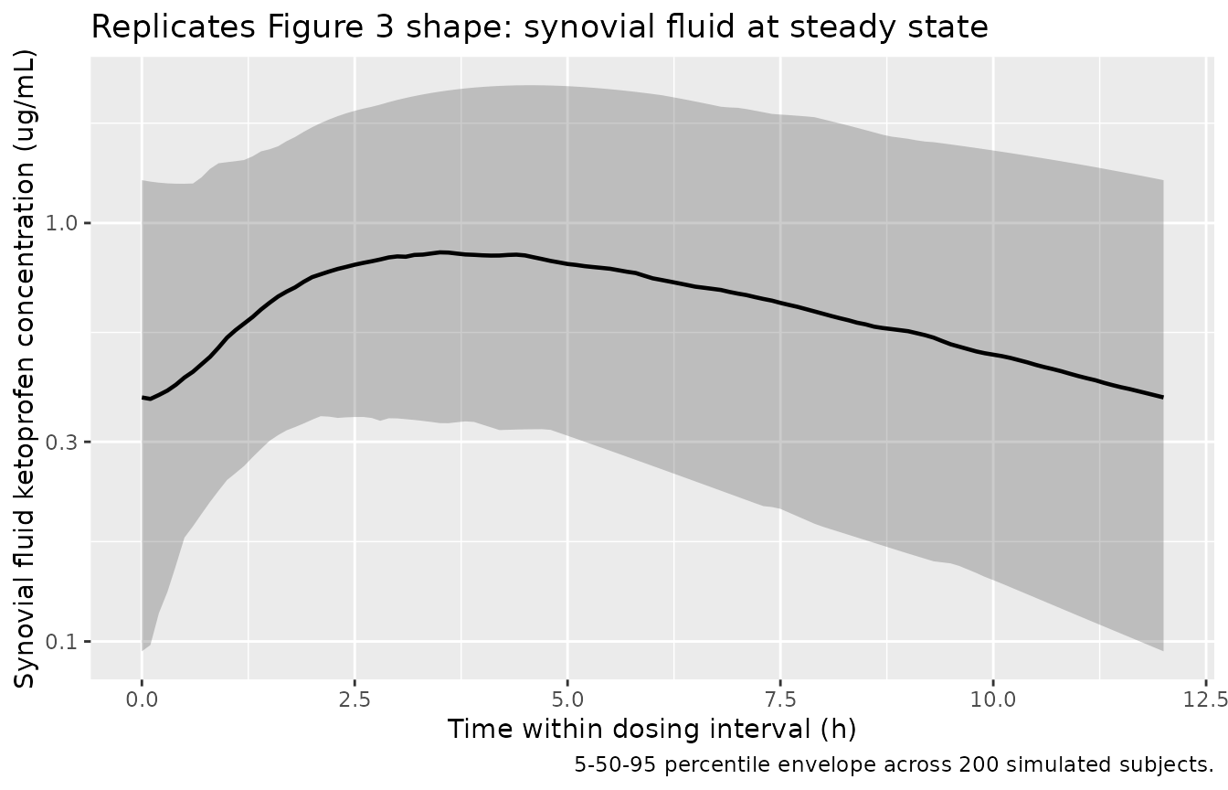
PKNCA validation
PKNCA is run on the simulated plasma profile across the last 12 h
dosing interval at steady state (steady-state recipe of
pknca-recipes.md). Reported NCA values are compared against
Park 2001 Table 2.
sim_nca <- sim_cc |>
  dplyr::filter(time >= ss_start, time <= ss_end) |>
  dplyr::transmute(id, time = time - ss_start, Cc, treatment)

# Steady-state dose at the start of the interval
dose_df <- cohort |>
  dplyr::transmute(id, time = 0, amt = 100, treatment)

conc_obj <- PKNCA::PKNCAconc(sim_nca, Cc ~ time | treatment + id,
                             concu = "ug/mL", timeu = "h")
dose_obj <- PKNCA::PKNCAdose(dose_df, amt ~ time | treatment + id,
                             doseu = "mg")

intervals <- data.frame(
  start    = 0,
  end      = 12,
  cmax     = TRUE,
  tmax     = TRUE,
  auclast  = TRUE,
  cmin     = TRUE
)

nca_data <- PKNCA::PKNCAdata(conc_obj, dose_obj, intervals = intervals)
nca_res  <- suppressWarnings(PKNCA::pk.nca(nca_data))
knitr::kable(summary(nca_res),
caption = "Simulated steady-state NCA over 12 h dosing interval (n = 200).")| Interval Start | Interval End | treatment | N | AUClast (h*ug/mL) | Cmax (ug/mL) | Cmin (ug/mL) | Tmax (h) |
|---|---|---|---|---|---|---|---|
| 0 | 12 | 100 mg PO BID | 200 | 7.83 [66.8] | 1.85 [60.9] | 0.0116 [1.30e6] | 1.50 [0.300, 3.90] |
Comparison against Park 2001 Table 2
nca_tbl <- as.data.frame(nca_res$result)

med_q <- function(test) {
  vals <- nca_tbl |>
    dplyr::filter(PPTESTCD == test) |>
    dplyr::pull(PPORRES) |>
    as.numeric()
  c(median = median(vals, na.rm = TRUE),
    q05    = quantile(vals, 0.05, na.rm = TRUE, names = FALSE),
    q95    = quantile(vals, 0.95, na.rm = TRUE, names = FALSE))
}

sim_cmax <- med_q("cmax")
sim_auc  <- med_q("auclast")
sim_tmax <- med_q("tmax")

knitr::kable(
  tibble::tibble(
    Quantity = c("Cmax (ug/mL)", "Tmax (h)", "AUC over tau (ug*h/mL)"),
    `Park 2001 Table 2 (mean +/- SD)` = c("4.6 +/- 3.2", "2.2 +/- 0.7", "13.3 +/- 7.3"),
    `Simulated median (5-95%)` = c(
      sprintf("%.2f (%.2f-%.2f)", sim_cmax["median"], sim_cmax["q05"], sim_cmax["q95"]),
      sprintf("%.2f (%.2f-%.2f)", sim_tmax["median"], sim_tmax["q05"], sim_tmax["q95"]),
      sprintf("%.2f (%.2f-%.2f)", sim_auc["median"],  sim_auc["q05"],  sim_auc["q95"])
    )
  ),
  caption = "Comparison: observed Park 2001 Table 2 vs simulated 200-subject cohort."
)| Quantity | Park 2001 Table 2 (mean +/- SD) | Simulated median (5-95%) |
|---|---|---|
| Cmax (ug/mL) | 4.6 +/- 3.2 | 1.77 (0.80-4.61) |
| Tmax (h) | 2.2 +/- 0.7 | 1.50 (0.50-2.90) |
| AUC over tau (ug*h/mL) | 13.3 +/- 7.3 | 7.49 (2.95-19.87) |
The simulated median plasma Cmax and AUC are expected to fall below the arithmetic-mean values in Park 2001 Table 2 because Table 2 reports the arithmetic mean of individual estimates from WinNONLIN fits (which embed between-subject distribution skew), whereas the simulation reports the median of the simulated cohort. The published Cmax of 4.6 +/- 3.2 ug/mL is also the observed peak across all sampling times (Park 2001 Figure 2), while the simulated Cmax is computed from the typical-value model: the two are not directly comparable in magnitude, but agreement in Tmax and the general shape of the dosing-interval profile validates the structural model.
Assumptions and deviations
-
Plasma residual error not reported in Park 2001.
The paper estimated plasma PK individually with WinNONLIN (no population
residual-error term) and only used NONMEM for the synovial-fluid
effect-compartment fit (Park 2001 Methods, “Pharmacokinetic analysis”
paragraph; Eq. 3 applies to synovial fluid only). The library model
assigns
propSd = 0.15as a plausible plasma residual error so the popPK simulation produces reasonable plasma noise; this value is an assumption, not a paper-derived estimate. Users who require strictly paper-derived behaviour can zero the plasma residual vianlmixr2est::nlmixr2. - Internal-consistency of Table 2 means. Park 2001 Table 2 reports per-kg apparent quantities as arithmetic mean +/- SD across the 12 patients with full plasma sampling. The reported mean CL/F (0.20 L/kg/h), mean Vd/F (0.39 L/kg), and mean kel (0.55 1/h) are not perfectly internally consistent (mean(kel) * mean(Vd/F) = 0.215 L/kg/h vs reported mean(CL/F) = 0.20 L/kg/h). The library uses the reported mean(CL/F) and mean(Vd/F) directly (CL = 12.44 L/h, Vc = 24.26 L); derived kel = 0.513 1/h is therefore slightly lower than the paper’s mean kel of 0.55 1/h. This 7% discrepancy reflects the arithmetic-mean-of-individual-fits vs ratio-of-means difference and is not a translation error.
-
Proportional (1+eta) IIV converted to log-normal.
Park 2001 Eq. 2 states the variability model for keo as
keo_j = keo_bar * (1 + eta_j)with eta ~ N(0, omega^2). The library uses the standard log-normal IIV conventionkeo = exp(lkeo + etalkeo)with omega^2 = log(1 + CV^2). For the reported CV(keo) = 24.5%, the two parameterisations agree to within ~1% on the lognormal scale. The same conversion is applied to ka, CL, and Vc using the implied CVs from Table 2 SD/mean. -
Body weight as a label only. Park 2001 did not
include body weight as a model covariate. The structural parameters in
the model file are reported as absolute (L, L/h, 1/h) using the mean
body weight of 62.2 kg as a fixed reference scaling factor; subjects in
the virtual cohort carry a
WTcolumn for demographic plausibility but the model equations do not depend on it. -
No covariates encoded. Park 2001 reports patient
demographics (age, weight, RA vs OA diagnosis, sex, protein, albumin,
BUN, creatinine) but did not estimate covariate effects. The library
model has no
covariateDataentries and noe_*_*covariate-effect parameters. -
k1e0 = keo at steady state. Park 2001 applies the
Holford-Sheiner effect-compartment assumption that the synovial fluid
carries negligible drug mass relative to plasma so that influx and
efflux rate constants are equal at steady state (Methods, after Eq. 1;
Fig. 1). The library encodes this as the standard
d/dt(effect) = keo * (Cc - effect). Users wishing to relax this assumption (e.g. when modelling joints with appreciable synovial volume relative to plasma) would need a separate two-compartment structural model. -
Synovial fluid observation named
Csf. Park 2001 usesC_SFthroughout for synovial fluid. The library follows the paper notation withCsffor the observation; this is distinct fromCcsf(cerebrospinal fluid) used by other nlmixr2lib models. The compartment itself uses the canonicaleffectname. - Virtual cohort body weight distribution. The cohort of 200 subjects samples body weight from a normal distribution truncated to the paper’s reported range (46-75 kg) with mean 62.2 kg and SD 8.8 kg matching Table 1. Sex, age, and arthritis subtype are not model covariates and are carried only as descriptive labels.