Rifapentine and rifabutin in mice (Chang 2023)
Source:vignettes/articles/Chang_2023_rifapentine_rifabutin_mouse.Rmd
Chang_2023_rifapentine_rifabutin_mouse.RmdModel and source
- Citation: Chang YS, Li SY, Pertinez H, Betoudji F, Lee J, Rannard SP, Owen A, Nuermberger EL, Ammerman NC. Using Dynamic Oral Dosing of Rifapentine and Rifabutin to Simulate Exposure Profiles of Long-Acting Formulations in a Mouse Model of Tuberculosis Preventive Therapy. Antimicrob Agents Chemother. 2023;67(7):e00481-23. doi:10.1128/aac.00481-23.
- Rifapentine model: Preclinical (mouse). One-compartment PK model with first-order oral absorption for rifapentine in female BALB/c mice of the paucibacillary tuberculosis-preventive-therapy model, dosed orally twice daily on a tapered schedule designed to mimic the exposure profile of a long-acting injectable (Chang 2023, second PK/PD study). Apparent clearance increases geometrically by a fixed fraction per dosing day (autoinduction, CL/F on dosing day n = CL/F on day 1 x (1 + Ind_Factor)^(n - 1)). Parameters were fitted per regimen to naive-pooled mouse plasma concentrations by weighted least squares (no between-subject variability); the default values are the ‘LAI target 0.6 ug/mL, 2 doses’ regimen fit, and the other regimen fits and the pilot / first-study fits (no induction term) are tabulated in the ini() comments and the vignette.
- Rifabutin model: Preclinical (mouse). One-compartment PK model with first-order oral absorption for rifabutin in female BALB/c mice of the paucibacillary tuberculosis-preventive-therapy model, dosed orally twice daily on a tapered schedule designed to mimic the exposure profile of a long-acting injectable (Chang 2023, second PK/PD study). Apparent clearance increases geometrically by a fixed fraction per dosing day (autoinduction, CL/F on dosing day n = CL/F on day 1 x (1 + Ind_Factor)^(n - 1)). Parameters were fitted to naive-pooled mouse plasma concentrations by weighted least squares (no between-subject variability); the default values are the ‘LAI target 0.15 ug/mL, 1 dose’ regimen fit, the only rifabutin regimen of that study that could be fitted, and the pilot / first-study fits (no induction term) are tabulated in the ini() comments and the vignette.
- Article: Antimicrob Agents Chemother. 2023;67(7):e00481-23 (open access, PMC10353356, with supplemental material)
Chang et al. used oral dosing of rifapentine (RPT) and rifabutin (RFB) in mice to mimic the plasma exposure profiles that a long-acting injectable (LAI) formulation might produce, and measured the bactericidal activity of those profiles in a paucibacillary mouse model of tuberculosis preventive therapy. Every PK analysis in the paper uses the same structure – a one-compartment model with first-order absorption, parameterised as CL/F, V/F and Ka – fitted separately to each dose group or regimen. The second PK/PD study, which ran for 8 weeks, added a time-dependent increase in CL/F that the authors attribute to rifamycin autoinduction:
The two packaged models carry that full structure, one per drug, with
the second-study fits as their default values. The pilot and first-study
fits are the same model with the induction factor absent, so this
vignette reproduces them by overriding the ini() values and
setting cl_time_fday = 0.
Population
All animals were BALB/c mice from Charles River Laboratories, dosed by oral gavage in 0.2 mL with doses computed for an average body mass of 20 g.
- Pilot PK study (Table 1, Table S2). 84 female and 48 male uninfected mice, 8-10 weeks old, 12 per dose group. Rifapentine 0.1, 0.3, 1 and 3 mg/kg and rifabutin 0.3, 1 and 3 mg/kg once daily in females (0.3 and 3 mg/kg of each drug in males), Monday to Friday in week 1 and Monday to Thursday in week 2 (nine doses). Staggered mandibular bleeds at 0, 0.5, 1, 2, 4, 6, 9 and 24 h after the first (day 0) and ninth (day 10) dose.
- PK/PD study 1 (Tables 2-3, Figs. S3 and S5). 125 female mice in the paucibacillary model (rBCG30 immunization, M. tuberculosis H37Rv challenge, treatment 7 weeks later). Twice-daily (BID) regimens designed to hold the plasma trough or average concentration at a target, 7 days per week for 3 weeks; every rifapentine regimen started with a loading dose.
- PK/PD study 2 (Tables 4-5, Table S5, Fig. 2, Fig. S7). 147 female mice in the same model. Twice-daily oral doses changed every 4 days over 8 weeks to trace the rise and slow decline of a simulated LAI injection (one simulated injection, or two given 4 weeks apart).
All fits pooled the individual mouse concentrations naively and
minimised least squares weighted by 1/(predicted)^2 (R 4.0.3,
pracma::lsqnonlin), so the models carry no between-subject
variability and the residual magnitude was not reported. The same
information is stored in the population metadata of each
model.
Source trace
| Item | Value | Source |
|---|---|---|
| Structure: 1-compartment, first-order absorption, CL/F, V/F, Ka | – | Methods, PK and PK/PD analyses |
Induction equation
CL/F(day n) = CL/F(day 1) x (1 + Ind_Factor)^(n - 1)
|
– | Methods (equation image m001) |
Day index: dosing day n - 1 = floor(t / 24)
|
– | Table 4 footnote b and Methods: all regimens dosed 7 days per week from day 0 |
RPT lka
|
log(0.42) | Table 5, LAI target 0.6 ug/mL, 2 doses |
RPT lcl
|
log(0.02) | Table 5, LAI target 0.6 ug/mL, 2 doses |
RPT lvc
|
log(0.35) | Table 5, LAI target 0.6 ug/mL, 2 doses |
RPT cl_time_fday
|
0.011 | Table 5, LAI target 0.6 ug/mL, 2 doses (Ind_Factor 1.1%) |
RFB lka
|
log(10.03) | Table 5, LAI target 0.15 ug/mL, 1 dose |
RFB lcl
|
log(1.06) | Table 5, LAI target 0.15 ug/mL, 1 dose |
RFB lvc
|
log(13.23) | Table 5, LAI target 0.15 ug/mL, 1 dose |
RFB cl_time_fday
|
0.009 | Table 5, LAI target 0.15 ug/mL, 1 dose (Ind_Factor 0.9%) |
propSd (both) |
fixed(0) | Methods: 1/pred^2 weighting; magnitude not reported |
| Other study-2 regimen fits | see below | Table 5 |
| Pilot fits, female | see below | Table 1 |
| Pilot fits, male | see below | Table S2 |
| Study-1 fits | see below | Fig. S3 (RPT) and Fig. S5 (RFB) panel tables |
| Study-2 dosing schedules | see below | Table S5 |
The rifapentine default is the “LAI target 0.6 ug/mL, 2 doses” fit because it has the lowest relative standard error on every parameter of the five rifapentine regimens; rifabutin has a single fitted study-2 regimen.
mod_rpt <- readModelDb("Chang_2023_rifapentine_mouse")
mod_rfb <- readModelDb("Chang_2023_rifabutin_mouse")
mods <- list(RPT = mod_rpt, RFB = mod_rfb)

# Solve one regimen with a given set of parameter estimates; Cc is the
# typical-value prediction (the models carry no random effects).
solve_fit <- function(drug, cl, v, ka, fday, events) {
  out <- rxode2::rxSolve(
    mods[[drug]],
    events,
    params = c(lcl = log(cl), lvc = log(v), lka = log(ka), cl_time_fday = fday),
    returnType = "data.frame"
  )
  out[!duplicated(out$time), c("time", "Cc")]
}

trap_auc <- function(time, conc) {
  sum(diff(time) * (head(conc, -1) + tail(conc, -1)) / 2)
}
Pilot PK study (Table 1 and Table S2)
Each pilot dose group was fitted separately with no induction term, to the day-0 and day-10 data together (the Fig. S3 caption describes the pilot model as fitted “including Day 10 PK data”; Table 1 and Table S2 print one parameter set per dose group). The simulation below reproduces the pilot schedule – nine once-daily doses on days 0-4 and 7-10 – with each group’s own fit and runs PKNCA on the 24-h interval after the first (day 0) and ninth (day 10) dose. The reference values are the paper’s observed Cmax and AUC0-24 from the naive-pooled data, so the comparison is “fitted model versus data”.
pilot <- tibble::tribble(
  ~drug, ~sex,     ~dose, ~cl,   ~v,    ~ka,
  "RPT", "female", 0.1,   0.024, 0.743, 2.57,
  "RPT", "female", 0.3,   0.029, 0.736, 1.75,
  "RPT", "female", 1,     0.021, 0.643, 1.64,
  "RPT", "female", 3,     0.016, 0.418, 1.33,
  "RFB", "female", 0.3,   0.674, 7.360, 49.10,
  "RFB", "female", 1,     1.040, 7.490, 16.40,
  "RFB", "female", 3,     1.170, 8.670, 8.48,
  "RPT", "male",   0.3,   0.020, 0.449, 1.05,
  "RPT", "male",   3,     0.015, 0.287, 0.75,
  "RFB", "male",   0.3,   1.39,  9.87,  48.9,
  "RFB", "male",   3,     1.79,  11.0,  47.7
) |>
  mutate(group = sprintf("%s %s mg/kg (%s)", drug, dose, sex))

# Observed NCA, Table 1 (female) and Table S2 (male): day 0 then day 10.
pilot_ref <- tibble::tribble(
  ~group,                   ~day, ~cmax,  ~auclast,
  "RPT 0.1 mg/kg (female)", 0,    0.130,  2.5,
  "RPT 0.1 mg/kg (female)", 10,   0.199,  3.6,
  "RPT 0.3 mg/kg (female)", 0,    0.386,  6.4,
  "RPT 0.3 mg/kg (female)", 10,   0.644,  9.6,
  "RPT 1 mg/kg (female)",   0,    1.580,  23.9,
  "RPT 1 mg/kg (female)",   10,   2.370,  38.7,
  "RPT 3 mg/kg (female)",   0,    6.690,  105.7,
  "RPT 3 mg/kg (female)",   10,   11.900, 166.6,
  "RFB 0.3 mg/kg (female)", 0,    0.053,  0.4,
  "RFB 0.3 mg/kg (female)", 10,   0.041,  0.3,
  "RFB 1 mg/kg (female)",   0,    0.140,  1.0,
  "RFB 1 mg/kg (female)",   10,   0.105,  0.8,
  "RFB 3 mg/kg (female)",   0,    0.325,  2.7,
  "RFB 3 mg/kg (female)",   10,   0.348,  2.4,
  "RPT 0.3 mg/kg (male)",   0,    0.491,  6.7,
  "RPT 0.3 mg/kg (male)",   10,   0.768,  10.5,
  "RPT 3 mg/kg (male)",     0,    10.6,   118.2,
  "RPT 3 mg/kg (male)",     10,   7.87,   159.8,
  "RFB 0.3 mg/kg (male)",   0,    0.034,  0.2,
  "RFB 0.3 mg/kg (male)",   10,   0.027,  0.2,
  "RFB 3 mg/kg (male)",     0,    0.299,  1.8,
  "RFB 3 mg/kg (male)",     10,   0.243,  1.6
) |>
  mutate(treatment = sprintf("%s, day %d", group, day))

pilot_dose_days <- c(0:4, 7:10)
sampling_times <- c(0, 0.5, 1, 2, 4, 6, 9, 24)

pilot_sim <- bind_rows(lapply(seq_len(nrow(pilot)), function(i) {
  r <- pilot[i, ]
  ev <- rxode2::et(amt = r$dose, cmt = "depot", time = pilot_dose_days * 24) |>
    rxode2::et(c(sampling_times, 240 + sampling_times), cmt = "central")
  s <- solve_fit(r$drug, r$cl, r$v, r$ka, 0, ev)
  bind_rows(
    mutate(filter(s, time <= 24), day = 0L),
    mutate(filter(s, time >= 240, time <= 264), day = 10L, time = time - 240)
  ) |>
    mutate(group = r$group, treatment = sprintf("%s, day %d", r$group, day), id = i)
}))
conc_obj <- PKNCA::PKNCAconc(
  dplyr::filter(pilot_sim, !is.na(Cc)),
  Cc ~ time | treatment + id
)
dose_df <- pilot_sim |>
  distinct(treatment, id) |>
  left_join(distinct(pilot_sim, treatment, group), by = "treatment") |>
  left_join(select(pilot, group, dose), by = "group") |>
  mutate(time = 0)
dose_obj <- PKNCA::PKNCAdose(dose_df, dose ~ time | treatment + id)
intervals <- data.frame(start = 0, end = 24, cmax = TRUE, tmax = TRUE, auclast = TRUE)
nca_res <- PKNCA::pk.nca(PKNCA::PKNCAdata(conc_obj, dose_obj, intervals = intervals))

pilot_cmp <- ncaComparisonTable(
  nca_res,
  as.data.frame(select(pilot_ref, treatment, cmax, auclast)),
  by = "treatment",
  params = c("cmax", "auclast"),
  tolerance_pct = 30,
  units = c(cmax = "ug/mL", auclast = "ug*h/mL")
)
knitr::kable(pilot_cmp, caption = "Pilot study Cmax and AUC0-24 after the day-0 and day-10 doses: simulated from each dose group's own fit (Table 1 / Table S2) versus the paper's observed values.")| NCA parameter | treatment | Reference | Simulated | % diff |
|---|---|---|---|---|
| Cmax (ug/mL) | RPT 0.1 mg/kg (female), day 0 | 0.13 | 0.127 | -2.3% |
| Cmax (ug/mL) | RPT 0.1 mg/kg (female), day 10 | 0.199 | 0.228 | +14.4% |
| Cmax (ug/mL) | RPT 0.3 mg/kg (female), day 0 | 0.386 | 0.373 | -3.4% |
| Cmax (ug/mL) | RPT 0.3 mg/kg (female), day 10 | 0.644 | 0.605 | -6.0% |
| Cmax (ug/mL) | RPT 1 mg/kg (female), day 0 | 1.58 | 1.43 | -9.7% |
| Cmax (ug/mL) | RPT 1 mg/kg (female), day 10 | 2.37 | 2.58 | +8.9% |
| Cmax (ug/mL) | RPT 3 mg/kg (female), day 0 | 6.69 | 6.33 | -5.4% |
| Cmax (ug/mL) | RPT 3 mg/kg (female), day 10 | 11.9 | 10.6 | -10.7% |
| Cmax (ug/mL) | RFB 0.3 mg/kg (female), day 0 | 0.053 | 0.039 | -26.4% |
| Cmax (ug/mL) | RFB 0.3 mg/kg (female), day 10 | 0.041 | 0.0439 | +7.0% |
| Cmax (ug/mL) | RFB 1 mg/kg (female), day 0 | 0.14 | 0.126 | -10.3% |
| Cmax (ug/mL) | RFB 1 mg/kg (female), day 10 | 0.105 | 0.13 | +24.0% |
| Cmax (ug/mL) | RFB 3 mg/kg (female), day 0 | 0.325 | 0.324 | -0.4% |
| Cmax (ug/mL) | RFB 3 mg/kg (female), day 10 | 0.348 | 0.337 | -3.2% |
| Cmax (ug/mL) | RPT 0.3 mg/kg (male), day 0 | 0.491 | 0.573 | +16.8% |
| Cmax (ug/mL) | RPT 0.3 mg/kg (male), day 10 | 0.768 | 0.875 | +13.9% |
| Cmax (ug/mL) | RPT 3 mg/kg (male), day 0 | 10.6 | 8.56 | -19.3% |
| Cmax (ug/mL) | RPT 3 mg/kg (male), day 10 | 7.87 | 12.1 | +54.0%* |
| Cmax (ug/mL) | RFB 0.3 mg/kg (male), day 0 | 0.034 | 0.0284 | -16.4% |
| Cmax (ug/mL) | RFB 0.3 mg/kg (male), day 10 | 0.027 | 0.0294 | +8.9% |
| Cmax (ug/mL) | RFB 3 mg/kg (male), day 0 | 0.299 | 0.252 | -15.6% |
| Cmax (ug/mL) | RFB 3 mg/kg (male), day 10 | 0.243 | 0.257 | +6.0% |
| AUClast (ug*h/mL) | RPT 0.1 mg/kg (female), day 0 | 2.5 | 2.21 | -11.4% |
| AUClast (ug*h/mL) | RPT 0.1 mg/kg (female), day 10 | 3.6 | 4.01 | +11.3% |
| AUClast (ug*h/mL) | RPT 0.3 mg/kg (female), day 0 | 6.4 | 6.21 | -3.0% |
| AUClast (ug*h/mL) | RPT 0.3 mg/kg (female), day 10 | 9.6 | 10.1 | +5.3% |
| AUClast (ug*h/mL) | RPT 1 mg/kg (female), day 0 | 23.9 | 25.3 | +6.0% |
| AUClast (ug*h/mL) | RPT 1 mg/kg (female), day 10 | 38.7 | 45.8 | +18.4% |
| AUClast (ug*h/mL) | RPT 3 mg/kg (female), day 0 | 106 | 110 | +4.0% |
| AUClast (ug*h/mL) | RPT 3 mg/kg (female), day 10 | 167 | 183 | +9.8% |
| AUClast (ug*h/mL) | RFB 0.3 mg/kg (female), day 0 | 0.4 | 0.386 | -3.4% |
| AUClast (ug*h/mL) | RFB 0.3 mg/kg (female), day 10 | 0.3 | 0.436 | +45.2%* |
| AUClast (ug*h/mL) | RFB 1 mg/kg (female), day 0 | 1 | 0.901 | -9.9% |
| AUClast (ug*h/mL) | RFB 1 mg/kg (female), day 10 | 0.8 | 0.936 | +17.0% |
| AUClast (ug*h/mL) | RFB 3 mg/kg (female), day 0 | 2.7 | 2.41 | -10.6% |
| AUClast (ug*h/mL) | RFB 3 mg/kg (female), day 10 | 2.4 | 2.52 | +4.8% |
| AUClast (ug*h/mL) | RPT 0.3 mg/kg (male), day 0 | 6.7 | 9.57 | +42.8%* |
| AUClast (ug*h/mL) | RPT 0.3 mg/kg (male), day 10 | 10.5 | 14.8 | +40.5%* |
| AUClast (ug*h/mL) | RPT 3 mg/kg (male), day 0 | 118 | 138 | +16.5% |
| AUClast (ug*h/mL) | RPT 3 mg/kg (male), day 10 | 160 | 198 | +23.8% |
| AUClast (ug*h/mL) | RFB 0.3 mg/kg (male), day 0 | 0.2 | 0.201 | +0.7% |
| AUClast (ug*h/mL) | RFB 0.3 mg/kg (male), day 10 | 0.2 | 0.209 | +4.4% |
| AUClast (ug*h/mL) | RFB 3 mg/kg (male), day 0 | 1.8 | 1.58 | -12.2% |
| AUClast (ug*h/mL) | RFB 3 mg/kg (male), day 10 | 1.6 | 1.61 | +0.8% |
pilot_nca <- as.data.frame(nca_res) |>
  filter(PPTESTCD %in% c("cmax", "auclast")) |>
  select(treatment, PPTESTCD, sim = PPORRES) |>
  left_join(
    pivot_longer(select(pilot_ref, treatment, cmax, auclast), -treatment,
      names_to = "PPTESTCD", values_to = "ref"
    ),
    by = c("treatment", "PPTESTCD")
  ) |>
  mutate(pct_diff = 100 * (sim - ref) / ref)
pilot_auc <- filter(pilot_nca, PPTESTCD == "auclast")
pilot_auc_female <- filter(pilot_auc, grepl("female", treatment))
stopifnot(
  nrow(pilot_nca) == 2 * nrow(pilot_ref),
  # Centre: a mis-transcribed CL/F or V/F moves a group by tens of percent.
  abs(median(pilot_nca$pct_diff)) < 10,
  median(abs(pilot_auc$pct_diff)) < 15,
  # Envelope over the main-text (Table 1, female) groups.
  quantile(abs(pilot_auc_female$pct_diff), 0.9) < 25
)
Simulating the whole nine-dose schedule reproduces the day-0 to day-10 rise in rifapentine exposure that the Results describe (Cmax and AUC0-24 about 1.5- to 1.6-fold higher on day 10): with half-lives of 18-21 h and once-daily dosing, rifapentine accumulates, so a single time-invariant fit per group spans both days. For the Table 1 (female) groups the fitted AUC0-24 is within 20% of the observed value in all but one interval. The exceptions, all visible in the table above, are properties of the published fits rather than of the implementation:
- RFB 0.3 mg/kg (female), day 10: the observed AUC0-24 of 0.3 ug*h/mL is near the 0.05 ug/mL limit of quantification, while the same fit matches day 0. The day-0 Cmax of that group is also below the observed value, because with Ka near 50 1/h the fitted curve peaks before the first 0.5-h sample.
- RPT 0.3 mg/kg (male): the Table S2 fit (CL/F 0.020 L/h/kg, V/F 0.449 L/kg, Ka 1.05 1/h) gives about 40% more AUC0-24 than observed on both days. The printed half-life of 15.6 h equals 0.693 x V/F / CL/F, so the three printed values are mutually consistent and there is no single-value transcription error to correct; the fit simply does not reproduce the reported NCA.
- RPT 3 mg/kg (male), day 10: observed Cmax (7.87 ug/mL) is lower than on day 0 (10.6 ug/mL) with a Tmax of 9 h, a profile a one-compartment first-order absorption model cannot follow.
PK/PD study 1: steady target concentrations (Table 3, Figs. S3 and S5)
Twice-daily doses were given at 7 am and 5 pm (10 h and 14 h apart; Fig. S2 caption), and the rifapentine regimens opened with a loading dose in place of the first maintenance dose. Each regimen’s fitted CL/F, V/F and Ka are printed beneath its panel in Fig. S3 (rifapentine) or Fig. S5 (rifabutin). Table 3 reports the average and trough concentrations of each fitted curve, which the simulation below recomputes over day 19 (the last full day before week 3).
study1 <- tibble::tribble(
  ~drug, ~regimen,              ~load, ~maint, ~cl,  ~v,    ~ka,   ~cave_ref, ~ctrough_ref,
  "RPT", "RPT 0.075 mg/kg BID", 0.2,   0.075,  0.03, 1.47,  0.89,  0.20,      0.17,
  "RPT", "RPT 0.25 mg/kg BID",  0.625, 0.25,   0.03, 1.10,  1.01,  0.63,      0.54,
  "RPT", "RPT 0.75 mg/kg BID",  1.875, 0.75,   0.02, 0.88,  1.33,  2.98,      2.60,
  "RPT", "RPT 1.25 mg/kg BID",  3.125, 1.25,   0.02, 0.68,  0.81,  5.60,      4.90,
  "RFB", "RFB 0.75 mg/kg BID",  NA,    0.75,   0.77, 8.12,  25.33, 0.09,      0.04,
  "RFB", "RFB 1.5 mg/kg BID",   NA,    1.5,    0.88, 8.74,  23.40, 0.16,      0.07,
  "RFB", "RFB 2.5 mg/kg BID",   NA,    2.5,    0.93, 10.97, 25.23, 0.24,      0.12,
  "RFB", "RFB 5.5 mg/kg BID",   NA,    5.5,    0.86, 8.56,  24.09, 0.60,      0.25
)

bid_times <- sort(c((0:20) * 24, (0:20) * 24 + 10))

study1_sim <- bind_rows(lapply(seq_len(nrow(study1)), function(i) {
  r <- study1[i, ]
  amt <- rep(r$maint, length(bid_times))
  if (!is.na(r$load)) amt[1] <- r$load
  ev <- bind_rows(
    data.frame(id = 1, time = bid_times, amt = amt, evid = 1, cmt = "depot"),
    data.frame(id = 1, time = seq(0, 21 * 24, by = 0.1), amt = 0, evid = 0, cmt = "central")
  ) |>
    arrange(time, desc(evid))
  solve_fit(r$drug, r$cl, r$v, r$ka, 0, ev) |>
    mutate(regimen = r$regimen, drug = r$drug)
}))

study1_cmp <- study1_sim |>
  filter(time >= 19 * 24, time <= 20 * 24) |>
  group_by(regimen) |>
  summarise(cave_sim = trap_auc(time, Cc) / 24, ctrough_sim = min(Cc), .groups = "drop") |>
  inner_join(study1, by = "regimen") |>
  mutate(
    cave_pct = 100 * (cave_sim - cave_ref) / cave_ref,
    ctrough_pct = 100 * (ctrough_sim - ctrough_ref) / ctrough_ref
  )

study1_cmp |>
  arrange(match(regimen, study1$regimen)) |>
  transmute(
    Regimen = regimen,
    `Cave, Table 3 (ug/mL)` = cave_ref,
    `Cave, simulated` = signif(cave_sim, 3),
    `Cave % diff` = round(cave_pct, 1),
    `Ctrough, Table 3 (ug/mL)` = ctrough_ref,
    `Ctrough, simulated` = signif(ctrough_sim, 3),
    `Ctrough % diff` = round(ctrough_pct, 1)
  ) |>
knitr::kable(caption = "Average and trough concentrations of the study-1 fitted curves (Table 3) versus simulation with each regimen's Fig. S3 / Fig. S5 estimates.")| Regimen | Cave, Table 3 (ug/mL) | Cave, simulated | Cave % diff | Ctrough, Table 3 (ug/mL) | Ctrough, simulated | Ctrough % diff |
|---|---|---|---|---|---|---|
| RPT 0.075 mg/kg BID | 0.20 | 0.208 | 4.2 | 0.17 | 0.1840 | 8.2 |
| RPT 0.25 mg/kg BID | 0.63 | 0.694 | 10.2 | 0.54 | 0.5850 | 8.3 |
| RPT 0.75 mg/kg BID | 2.98 | 3.120 | 4.9 | 2.60 | 2.7000 | 3.7 |
| RPT 1.25 mg/kg BID | 5.60 | 5.210 | -7.0 | 4.90 | 4.3600 | -11.1 |
| RFB 0.75 mg/kg BID | 0.09 | 0.081 | -10.0 | 0.04 | 0.0380 | -5.0 |
| RFB 1.5 mg/kg BID | 0.16 | 0.142 | -11.4 | 0.07 | 0.0631 | -9.8 |
| RFB 2.5 mg/kg BID | 0.24 | 0.224 | -6.8 | 0.12 | 0.1150 | -4.4 |
| RFB 5.5 mg/kg BID | 0.60 | 0.532 | -11.3 | 0.25 | 0.2370 | -5.1 |
stopifnot(
  nrow(study1_cmp) == nrow(study1),
  abs(median(c(study1_cmp$cave_pct, study1_cmp$ctrough_pct))) < 10,
  max(abs(study1_cmp$cave_pct)) < 15,
  max(abs(study1_cmp$ctrough_pct)) < 15
)
Every average and trough concentration agrees within 15%. The residual differences are the size expected from the two-significant-figure CL/F values printed in Figs. S3 and S5 (for example, a printed rifapentine CL/F of 0.03 L/h/kg covers 0.025-0.035): the steady-state average concentration is the daily dose divided by 24 x CL/F, so it moves one-for-one with the rounding.
ggplot(study1_sim, aes(time / (24 * 7), Cc)) +
  geom_line(colour = "orange") +
  geom_hline(
    data = study1, aes(yintercept = ctrough_ref), colour = "red", linetype = "dashed"
  ) +
  facet_wrap(~regimen, scales = "free_y", ncol = 2) +
  scale_y_log10() +
  labs(
    x = "Weeks of dosing", y = "Plasma concentration (ug/mL)",
    title = "Study-1 fitted profiles (replicates the yellow curves of Figs. S3 and S5)",
    caption = "Dashed red line: fitted trough concentration from Table 3."
  ) +
  theme_bw()
#> Warning in scale_y_log10(): log-10 transformation introduced infinite values.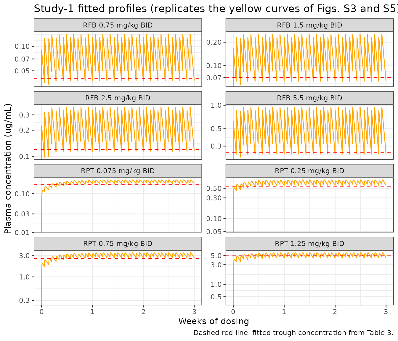
PK/PD study 2: simulated LAI profiles (Fig. 2, Table 5)
Table S5 lists the twice-daily dose for each of the 14 four-day periods of the 8-week course. The total doses it implies equal the Table 5 totals (35.4, 61.8, 74.0, 129.2 and 113.8 mg/kg for rifapentine; 254.8 mg/kg for the rifabutin regimen), which confirms the schedule is transcribed correctly. The two daily doses are placed 10 h and 14 h apart as in study 1. Each regimen is solved with its own Table 5 fit, including its induction factor.
table_s5 <- list(
  "RPT LAI 0.6 ug/mL, 1 dose" = c(0.75, 0.6, 0.5, 0.45, 0.375, 0.325, 0.275, 0.24, 0.21, 0.18, 0.16, 0.14, 0.12, 0.1),
  "RPT LAI 0.6 ug/mL, 2 doses" = c(0.75, 0.6, 0.5, 0.45, 0.375, 0.325, 0.275, 1, 0.8, 0.7, 0.6, 0.52, 0.45, 0.375),
  "RPT LAI 2 ug/mL, 1 dose" = c(1.6, 1.2, 1.1, 0.9, 0.8, 0.7, 0.6, 0.5, 0.425, 0.375, 0.325, 0.275, 0.25, 0.2),
  "RPT LAI 2 ug/mL, 2 doses" = c(1.6, 1.2, 1.1, 0.9, 0.8, 0.7, 0.6, 2.1, 1.625, 1.475, 1.225, 1.075, 0.95, 0.8),
  "RPT LAI 3.5 ug/mL, 1 dose" = c(2.4, 1.9, 1.6, 1.4, 1.2, 1.1, 0.875, 0.8, 0.7, 0.6, 0.5, 0.45, 0.375, 0.325),
  "RFB LAI 0.15 ug/mL, 1 dose" = c(5, 4, 3.5, 3, 2.75, 2.5, 2.2, 2, 1.6, 1.4, 1.2, 1, 0.9, 0.8)
)

study2 <- tibble::tribble(
  ~regimen,                     ~drug, ~cl,  ~v,    ~ka,   ~fday, ~total_ref, ~auc_ref, ~tr28_ref, ~tr52_ref,
  "RPT LAI 0.6 ug/mL, 1 dose",  "RPT", 0.02, 0.37,  0.23,  0.011, 35.4,       1320,     0.60,      0.15,
  "RPT LAI 0.6 ug/mL, 2 doses", "RPT", 0.02, 0.35,  0.42,  0.011, 61.8,       2093,     0.52,      0.45,
  "RPT LAI 2 ug/mL, 1 dose",    "RPT", 0.02, 0.64,  5.09,  0.011, 74.0,       3251,     1.58,      0.38,
  "RPT LAI 2 ug/mL, 2 doses",   "RPT", 0.02, 0.48,  0.62,  0.012, 129.2,      5074,     1.52,      1.37,
  "RPT LAI 3.5 ug/mL, 1 dose",  "RPT", 0.02, 0.45,  0.57,  0.011, 113.8,      5217,     2.32,      0.59,
  "RFB LAI 0.15 ug/mL, 1 dose", "RFB", 1.06, 13.23, 10.03, 0.009, 254.8,      200,      0.06,      0.02
)

study2$total_s5 <- vapply(study2$regimen, function(r) 8 * sum(table_s5[[r]]), numeric(1))
stopifnot(all(abs(study2$total_s5 - study2$total_ref) < 0.05))

study2_events <- function(regimen) {
  day_dose <- rep(table_s5[[regimen]], each = 4) # 14 periods x 4 days = 56 days
  am <- (0:55) * 24
  bind_rows(
    data.frame(id = 1, time = c(am, am + 10), amt = rep(day_dose, 2), evid = 1, cmt = "depot"),
    data.frame(
      id = 1, time = sort(unique(c(seq(0, 56 * 24, by = 0.25), 28 * 24, 52 * 24))),
      amt = 0, evid = 0, cmt = "central"
    )
  ) |>
    arrange(time, desc(evid))
}

study2_sim <- bind_rows(lapply(seq_len(nrow(study2)), function(i) {
  r <- study2[i, ]
  solve_fit(r$drug, r$cl, r$v, r$ka, r$fday, study2_events(r$regimen)) |>
    mutate(regimen = r$regimen)
}))
study2_sim |>
  filter(grepl("^RPT", regimen)) |>
  ggplot(aes(time / (24 * 7), Cc)) +
  geom_line(colour = "orange") +
  facet_wrap(~regimen, ncol = 2, scales = "free_y") +
  scale_y_log10() +
  scale_x_continuous(breaks = 0:8) +
  labs(
    x = "Weeks of dosing", y = "Plasma concentration (ug/mL)",
    title = "Rifapentine simulated-LAI regimens (replicates the yellow curves of Fig. 2A-E)"
  ) +
  theme_bw()
#> Warning in scale_y_log10(): log-10 transformation introduced infinite values.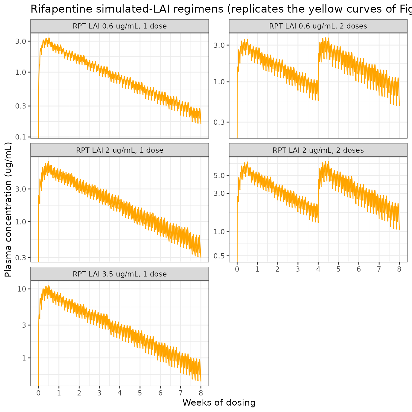
study2_sim |>
  filter(grepl("^RFB", regimen)) |>
  ggplot(aes(time / (24 * 7), Cc)) +
  geom_line(colour = "orange") +
  geom_hline(yintercept = 0.05, colour = "grey50", linetype = "dotted") +
  scale_y_log10() +
  scale_x_continuous(breaks = 0:8) +
  labs(
    x = "Weeks of dosing", y = "Plasma concentration (ug/mL)",
    title = "Rifabutin LAI target 0.15 ug/mL (replicates the yellow curve of Fig. S7D)",
    caption = "Dotted line: rifabutin LLOQ 0.05 ug/mL."
  ) +
  theme_bw()
#> Warning in scale_y_log10(): log-10 transformation introduced infinite values.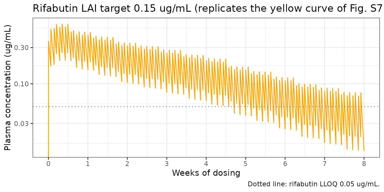
Cumulative AUC and troughs (Table 5)
Table 5 reports, for each regimen, the cumulative AUC of the fitted curve over the 8-week course and the fitted trough concentration on days 28 and 52 (taken here as the pre-morning-dose concentration on those days).
study2_cmp <- study2_sim |>
  group_by(regimen) |>
  summarise(
    auc_sim = trap_auc(time, Cc),
    tr28_sim = Cc[time == 28 * 24][1],
    tr52_sim = Cc[time == 52 * 24][1],
    .groups = "drop"
  ) |>
  inner_join(study2, by = "regimen") |>
  arrange(match(regimen, study2$regimen)) |>
  mutate(auc_pct = 100 * (auc_sim - auc_ref) / auc_ref)

study2_cmp |>
  transmute(
    Regimen = regimen,
    `Cum. AUC, Table 5 (ug*h/mL)` = auc_ref,
    `Cum. AUC, simulated` = round(auc_sim),
    `AUC % diff` = round(auc_pct, 1),
    `Day 28 trough, Table 5` = tr28_ref,
    `Day 28 trough, simulated` = signif(tr28_sim, 2),
    `Day 52 trough, Table 5` = tr52_ref,
    `Day 52 trough, simulated` = signif(tr52_sim, 2)
  ) |>
knitr::kable(caption = "Fitted cumulative AUC (0-8 weeks) and troughs of the study-2 regimens: Table 5 versus simulation with each regimen's Table 5 estimates.")| Regimen | Cum. AUC, Table 5 (ug*h/mL) | Cum. AUC, simulated | AUC % diff | Day 28 trough, Table 5 | Day 28 trough, simulated | Day 52 trough, Table 5 | Day 52 trough, simulated |
|---|---|---|---|---|---|---|---|
| RPT LAI 0.6 ug/mL, 1 dose | 1320 | 1457 | 10.3 | 0.60 | 0.66 | 0.15 | 0.200 |
| RPT LAI 0.6 ug/mL, 2 doses | 2093 | 2316 | 10.7 | 0.52 | 0.57 | 0.45 | 0.620 |
| RPT LAI 2 ug/mL, 1 dose | 3251 | 3034 | -6.7 | 1.58 | 1.40 | 0.38 | 0.400 |
| RPT LAI 2 ug/mL, 2 doses | 5074 | 4719 | -7.0 | 1.52 | 1.30 | 1.37 | 1.400 |
| RPT LAI 3.5 ug/mL, 1 dose | 5217 | 4674 | -10.4 | 2.32 | 1.90 | 0.59 | 0.560 |
| RFB LAI 0.15 ug/mL, 1 dose | 200 | 203 | 1.4 | 0.06 | 0.06 | 0.02 | 0.016 |
The rifabutin regimen, whose CL/F is printed to three significant figures, reproduces the published AUC within 2%. Every rifapentine CL/F in Table 5 is printed as 0.02 L/h/kg – one significant figure, compatible with any value from 0.015 to 0.025 – and the AUC scales almost inversely with CL/F, so the rifapentine AUC differences of up to about 11% are rounding, not structure. The check below makes this explicit: it back-solves, for each rifapentine regimen, the day-1 CL/F that reproduces the published cumulative AUC with all other parameters at their Table 5 values, and confirms that this CL/F rounds to the printed 0.02.
auc_for_cl <- function(cl, r) {
  s <- solve_fit(r$drug, cl, r$v, r$ka, r$fday, study2_events(r$regimen))
  trap_auc(s$time, s$Cc)
}

implied <- filter(study2, drug == "RPT")
implied$cl_implied <- vapply(seq_len(nrow(implied)), function(i) {
  r <- implied[i, ]
  uniroot(function(cl) auc_for_cl(cl, r) - r$auc_ref, interval = c(0.01, 0.04), tol = 1e-6)$root
}, numeric(1))

implied |>
  transmute(
    Regimen = regimen,
    `CL/F printed (L/h/kg)` = cl,
    `CL/F reproducing the Table 5 AUC` = signif(cl_implied, 3)
  ) |>
knitr::kable(caption = "Day-1 CL/F that reproduces each rifapentine regimen's published cumulative AUC.")| Regimen | CL/F printed (L/h/kg) | CL/F reproducing the Table 5 AUC |
|---|---|---|
| RPT LAI 0.6 ug/mL, 1 dose | 0.02 | 0.0221 |
| RPT LAI 0.6 ug/mL, 2 doses | 0.02 | 0.0222 |
| RPT LAI 2 ug/mL, 1 dose | 0.02 | 0.0186 |
| RPT LAI 2 ug/mL, 2 doses | 0.02 | 0.0186 |
| RPT LAI 3.5 ug/mL, 1 dose | 0.02 | 0.0179 |
stopifnot(
  all(round(implied$cl_implied, 2) == 0.02),
  abs(study2_cmp$auc_pct[study2_cmp$drug == "RFB"]) < 5,
  abs(median(study2_cmp$auc_pct)) < 10
)
Every implied CL/F lies between 0.018 and 0.022 L/h/kg, inside the rounding interval of the printed 0.02. The troughs follow the same pattern: they are within the range spanned by CL/F 0.015-0.025 but, being single-time-point values on a steep part of the curve, they are more sensitive to the rounding than the AUC is.
Induction factor
fold_day52 <- c(RPT = 1.011^51, RFB = 1.009^51)
fold_day52
#>      RPT      RFB
#> 1.747064 1.579245
stopifnot(all(abs(fold_day52 - c(1.75, 1.58)) < 0.01))
With CL/F on dosing day 52 equal to CL/F on day 1 times (1 + Ind_Factor)^51, the rifapentine factor of 1.1% per day gives a 1.75-fold higher clearance by day 52 and the rifabutin factor of 0.9% a 1.58-fold higher clearance, consistent with the Results’ “~1.7 times higher clearance by day 52 of the study than day 1”.
Pharmacodynamic summary (not encoded)
The paper summarises each regimen’s lung CFU time course with a “net bacterial elimination” rate constant, knet, estimated as the slope of a straight line through log10 CFU versus time (Methods; Table 3). These are per-arm descriptive slopes with no fitted exposure-response function linking them to concentration (Fig. S4 plots them against dose and exposure only), so they are reported here for reference rather than encoded as a PD model.
| Study-1 regimen | knet (1/week) [% RSE] | Initial log10 CFU/lung |
|---|---|---|
| Untreated | 0.05 [124] | 4.45 |
| Rifampin 10 mg/kg QD | -0.21 [32.88] | 4.45 |
| RPT 0.075 mg/kg BID | 0.12 [56.71] | 4.46 |
| RPT 0.25 mg/kg BID | 0.07 [98.28] | 4.44 |
| RPT 0.75 mg/kg BID | -0.22 [29.30] | 4.44 |
| RPT 1.25 mg/kg BID | -0.28 [23.20] | 4.45 |
| RFB 0.75 mg/kg BID | -0.09 [90.11] | 4.46 |
| RFB 1.5 mg/kg BID | -0.20 [39.48] | 4.46 |
| RFB 2.5 mg/kg BID | -0.30 [25.41] | 4.45 |
| RFB 5.5 mg/kg BID | -0.48 [15.86] | 4.45 |
Assumptions and deviations
-
Many fits, one structure. The paper fits its
one-compartment model separately to 25 dose groups and regimens. The
packaged models carry the second-study structure (with the induction
term) and one fit as defaults; every other fit is listed in the model
file comments and reproduced here by overriding the
ini()values, withcl_time_fday = 0for the pilot and study-1 fits, which had no induction term. - Choice of rifapentine defaults. The “LAI target 0.6 ug/mL, 2 doses” regimen was chosen because its estimates have the lowest relative standard errors of the five rifapentine regimens. CL/F (0.02) and Ind_Factor (1.1%) are the same, to the printed precision, in four of the five regimens; V/F and Ka vary more between regimens and are poorly determined in some (V/F RSE 122%, Ka RSE 129% for the single-dose 0.6 ug/mL regimen).
-
Day index. The induction equation counts dosing
days. All study-2 regimens were dosed every day from day 0, so dosing
day n - 1 is
floor(t / 24)witht = 0at the first dose. A user simulating a schedule with dosing-free days, or a first dose away fromt = 0, must account for this. -
Residual error. The fits minimised least squares
weighted by 1/(predicted)^2, which corresponds to a proportional error
model, but no residual magnitude is reported;
propSdis fixed at 0. - Near-zero RSE on Ka. Several rifabutin Ka estimates (and one rifapentine estimate, 5.09 1/h with an RSE of 0.004%) carry an RSE of about 0%. The paper never states that a parameter was fixed; the authors describe rifabutin absorption as very rapid at every dose, so the near-zero RSE reflects an absorption rate the 0.5-1 h earliest samples cannot inform. These values are treated as estimates, not fixed values.
- Dose timing. Twice-daily doses are placed 10 h and 14 h apart (7 am and 5 pm), as stated for study 1 in the Fig. S2 caption; the Methods give 12 +/- 2 h for both studies. The cumulative AUC and average concentration are insensitive to this choice.
- AUC window and trough day. Table 5 does not state the integration window of the “cumulative AUC”; the full 8-week (56-day) course is used. The day-28 and day-52 troughs are read at the pre-morning-dose time on those study days.
- Body weight. Doses and parameters are per kilogram; the paper dosed for an average mouse of 20 g and reports no weight effect.
- Rifabutin “LAI target 0.045 ug/mL” regimen. Not fitted by the authors (truncated PK profile, most samples below the LLOQ; Table 5 footnote f), so it has no parameter set to reproduce.