Benralizumab (Yan 2019) • nlmixr2lib

Model and source

Citation: Yan L, Wang B, Chia YL, Roskos LK. Population pharmacokinetic modeling of benralizumab in adult and adolescent patients with asthma. Clin Pharmacokinet. 2019;58(7):943-958. doi:10.1007/s40262-019-00738-4. Parameter values are the ‘Final updated model (Model 9)’ column of Table 5, the model refitted to all nine studies after ZONDA was appended to the analysis dataset. Superseded for the Asian and paediatric populations by Jin Y, Guiastrennec B, Stuke M, et al. Clin Pharmacokinet. 2025;64:1233-1245; doi:10.1007/s40262-025-01538-9 – see modellib(‘Jin_2025_benralizumab’).
Description: Two-compartment population PK model of benralizumab (anti-IL-5R alpha) with first-order subcutaneous absorption and first-order elimination in adult and adolescent patients with asthma (Yan 2019), pooling nine phase I-III studies; body weight on CL/Vc/Vp, anti-drug antibody on CL, a study-specific absolute subcutaneous bioavailability for the phase IIb study MI-CP220, and study-stratified log-scale residual error
Article: https://doi.org/10.1007/s40262-019-00738-4 (open access)

Benralizumab is an interleukin-5 receptor alpha-directed cytolytic monoclonal antibody approved as add-on maintenance treatment for patients aged 12 years and older with severe eosinophilic asthma. Yan 2019 is the pooled population PK analysis of the phase I-III programme that supported that registration.

Three benralizumab population PK models are packaged in nlmixr2lib and they are not interchangeable:

Model	Scope	Distinguishing features
`modellib("Wang_2017_benralizumab")`	Early-phase healthy volunteers and patients with asthma	Includes a PD (eosinophil) layer; the ADA covariate uses a HIGH-TITER (>= 400) definition; Japanese-heritage effect on Vc
`modellib("Yan_2019_benralizumab")` (this page)	Nine pooled phase I-III asthma studies, 2317 patients	The registrational PK model; plain positive/negative ADA; MI-CP220 study bioavailability stratum
`modellib("Jin_2025_benralizumab")`	Twelve pooled studies, 2855 participants, adding Chinese and paediatric data	Updates this model; adds an Asian-race effect on CL, an AMES study bioavailability stratum, and a 200 mg dose effect on F

Yan 2019 is the direct predecessor of Jin 2025, which calls it the “legacy model”. Where the two are compared below, the agreement is used as an independent check on how an ambiguous Yan 2019 table row should be read.

Population

The analysis pooled 2317 patients with asthma from 9 clinical studies (Yan 2019 Table 1): five phase I/II studies (NCT00512486, NCT00659659, NCT00768079, NCT00783289, and the phase IIb study NCT01238861, which the paper also calls MI-CP220 or “CP220”) and the four phase III studies SIROCCO (NCT01928771), CALIMA (NCT01914757), ZONDA (NCT02075255) and BISE (NCT02322775).

Baseline demographics come from Yan 2019 Tables 2 and 3: median age 50 years (range 12-75), of whom only 57 patients (2.46%) were adolescents aged 12-17; median body weight 77 kg (range 40-204.4); 63.96% female; 77.73% White, 9.8% Asian, 4.96% African American and 7.51% Other. Anti-drug antibodies were detected at some assessed visit in 362 patients (15.62%). No healthy volunteers were enrolled. Doses spanned 0.0003-3 mg/kg intravenously and 2-200 mg subcutaneously, but 80% of patients received the registrational 30 mg subcutaneous dose.

The final updated model was fitted to 14,918 quantifiable serum (plasma for NCT00659659) concentrations. ZONDA was first held out for external validation (Yan 2019 Results 3.4, Figure 2) and then appended for the final re-estimation (Results 3.5).

The same information is available programmatically:

str(readModelDb("Yan_2019_benralizumab")()$population, max.level = 1)
#> List of 14
#>  $ species       : chr "human"
#>  $ n_subjects    : int 2317
#>  $ n_studies     : int 9
#>  $ age_range     : chr "12-75 years (adults 18-75, n = 2260, 97.54%; adolescents 12-17, n = 57, 2.46%)"
#>  $ age_median    : chr "50 years (range 12-75); mean 48.48 +/- 13.88 years"
#>  $ weight_range  : chr "40-204.4 kg"
#>  $ weight_median : chr "77 kg (range 40-204.4); mean 79.14 +/- 19.74 kg over the 2316 patients with a recorded weight"
#>  $ sex_female_pct: num 64
#>  $ race_ethnicity: Named num [1:4] 77.73 4.96 9.8 7.51
#>   ..- attr(*, "names")= chr [1:4] "White" "African American" "Asian" "Other"
#>  $ disease_state : chr "Asthma. The five phase I/II studies enrolled patients with mild atopic, eosinophilic or uncontrolled asthma; th"| __truncated__
#>  $ dose_range    : chr "Per Yan 2019 Table 1. Intravenous, single dose: 0.0003-3 mg/kg (phase I NCT00512486), 1.0 mg/kg (phase I NCT006"| __truncated__
#>  $ regions       : chr "Multi-regional; nine AstraZeneca/MedImmune trials, the largest being SIROCCO (NCT01928771) and CALIMA (NCT01914757)."
#>  $ immunogenicity: chr "362 of 2317 patients (15.62%) were anti-drug antibody positive at some assessed visit."
#>  $ notes         : chr "14,918 quantifiable serum (plasma for NCT00659659) benralizumab concentrations from 2317 patients across all ni"| __truncated__

Source trace

Every value below is from the “Final updated model (Model 9)” column of Yan 2019 Table 5 unless stated otherwise. The base-model column of the same table belongs to Model 5, an earlier eight-study fit with no covariates, and is not used. The per-parameter origin is also recorded as an in-file comment beside each ini() entry in inst/modeldb/specificDrugs/Yan_2019_benralizumab.R.

Equation / parameter	Value in the model file	Source location
Two-compartment structure, first-order SC absorption, first-order elimination from central	`d/dt(depot)`, `d/dt(central)`, `d/dt(peripheral1)`	Methods 2.5.4 and Figure 1
`lcl`	`log(0.291)`	Table 5, “CL, L/day” = 0.291 (90% CI 0.28-0.302)
`lvc`	`log(3.13)`	Table 5, “Vc, L” = 3.13 (90% CI 2.97-3.31)
`lq`	`log(0.738)`	Table 5, “Q, L/day” = 0.738 (90% CI 0.679-0.803)
`lvp`	`log(2.52)`	Table 5, “Vp, L” = 2.52 (90% CI 2.34-2.71)
`lka`	`log(log(2) / 3.54)`	Table 5, “ka, half-life; days” = 3.54 (90% CI 3.15-3.99); the paper parameterises the absorption HALF-LIFE, so `ka` is derived
`lfdepot`	`log(0.589)`	Table 5, “F” = 0.589 (90% CI 0.565-0.614)
`lfdepot_micp220`	`log(0.490)`	Table 5, “Change in F with study CP220, fraction” = 0.490 (90% CI 0.461-0.522)
`e_wt_cl`	`0.807`	Table 5, “Body weight on CL, power”; the Figure 4 caption prints the curve as `CL.(body weight/70)^0.807`
`e_wt_vc`	`0.803`	Table 5, “Body weight on Vc, power” (90% CI 0.627-0.979)
`e_wt_vp`	`0.528`	Table 5, “Body weight on Vp, power” (90% CI 0.351-0.706)
(no weight effect on Q)	–	Table 5, “Body weight on Q, power” = 0 with no confidence interval, i.e. dropped by the Wald’s Approximation Method step of Methods 2.5.7
`e_ada_cl`	`log(2.24)`	Table 5, “ADAs on CL, fraction” = 2.24 (90% CI 2.18-2.3); the abstract and Discussion restate it as “+124%”
70 kg reference weight	`(WT / 70)^...`	Methods 2.5.6 (“70 kg for body weight”) and the Figure 4 caption
Power form for continuous covariates	`(WT / 70)^beta`	Equation 3
Fractional-change form for categorical covariates	`exp(beta * indicator)`	Equation 4
`etalcl`	`0.242^2`	Table 5, “etaCL, %CV” = 24.2
`etalvc`	`0.244^2`	Table 5, “etaVc, %CV” = 24.4
`etalq`	`fixed(0.008)`	Table 4, Model 8, “Fixed IIV(Q) = 0.008”; Table 5 prints the matching 8.94 %CV with no CI
`etalvp`	`0.447^2`	Table 5, “etaVp, %CV” = 44.7
`etalka`	`0.831^2`	Table 5, “etaka (half-life), %CV” = 83.1
`etalfdepot`	`0.171^2`	Table 5, “etaF, %CV” = 17.1
`etalfdepot_micp220`	`0.350^2`	Table 5, “etaF (study CP220), %CV” = 35.0
`expSd`	`0.367`	Table 5, “Proportional error (studies SIROCCO, CALIMA, ZONDA, BISE), %CV” = 36.7
`expSd_Cc_early`	`0.250`	Table 5, “Proportional error, %CV” = 25.0; Results 3.2 assigns this row to the phase I-IIa studies
`expSd_Cc_micp220`	`0.545`	Table 5, “Proportional error (study CP220), %CV” = 54.5
Log-normal residual error	`Cc ~ lnorm(...)`	Results 3.2, “the PK concentration data were log-transformed … A log-normal residual error structure was used”

Two table-reading decisions worth recording

Table 5 reports IIV as 100 * omega_SD, not as an exact lognormal CV. Table 4 states that Model 8 holds IIV(Q) = 0.008, which in NONMEM is an omega variance. Table 5 prints the corresponding etaQ as 8.94 %CV. Since 100 * sqrt(0.008) = 8.944 while the exact lognormal CV 100 * sqrt(exp(0.008) - 1) = 8.962 would have printed as 8.96, the tabulated percentages are standard deviations. nlmixr2’s ~ takes a variance, so each percentage is squared in the model file.

c(
  as_sd = 100 * sqrt(0.008),
  as_exact_lognormal_cv = 100 * sqrt(exp(0.008) - 1),
  printed_in_table_5 = 8.94
)
#>                 as_sd as_exact_lognormal_cv    printed_in_table_5 
#>              8.944272              8.962190              8.940000

The MI-CP220 bioavailability row is an ABSOLUTE fraction, not a multiplier. Table 5 labels the row “Change in F with study CP220, fraction”, which reads like the exp(theta) multiplier of Equation 4 – and for the row immediately above it (“ADAs on CL, fraction” = 2.24) that is exactly what it is. For F it is not, and three independent checks agree:

The base-model column of the same table gives 0.569 against a reference F of 0.671, a ratio of 0.848. The successor analysis Jin_2025_benralizumab refits the same MI-CP220 data and reports Fa1S220 / Fa1 = 0.457 / 0.539, which is also 0.848. Reading the Yan 2019 row as a multiplier would make the relative bioavailability 0.569, not 0.848.
The final-model ratio 0.490 / 0.589 = 0.832 stays in the same place. Under the multiplier reading the relative bioavailability would have moved from 0.569 to 0.490 between two fits of overlapping data.
The stratum carries its own separately tabulated IIV (“etaF (study CP220), %CV” = 35.0 versus 17.1 for the reference F). A separately estimated absolute fraction has its own omega; a shift applied to a shared parameter does not.

tibble::tibble(
  analysis = c(
    "Yan 2019 base model (Model 5)",
    "Yan 2019 final model (Model 9)",
    "Jin 2025 final model"
  ),
  f_reference = c(0.671, 0.589, 0.539),
  f_micp220 = c(0.569, 0.490, 0.457)
) |>
  mutate(ratio = round(f_micp220 / f_reference, 3)) |>
  knitr::kable(
    caption = paste(
      "MI-CP220 bioavailability relative to the reference studies. The ratios",
      "agree across two independent analyses of overlapping data, which the",
      "relative-multiplier reading of the Yan 2019 row could not produce."
    )
  )

MI-CP220 bioavailability relative to the reference studies. The ratios agree across two independent analyses of overlapping data, which the relative-multiplier reading of the Yan 2019 row could not produce.
analysis	f_reference	f_micp220	ratio
Yan 2019 base model (Model 5)	0.671	0.569	0.848
Yan 2019 final model (Model 9)	0.589	0.490	0.832
Jin 2025 final model	0.539	0.457	0.848

The three residual-error strata are read the same way, and corroborated the same way: Yan 2019 prints the phase III stratum as 36.7 %CV and Jin 2025 tabulates the same stratum as Error_ADD3, log(ng/mL) = 0.367.

Model structure

mod <- readModelDb("Yan_2019_benralizumab")
ui <- rxode2::rxode2(mod)
#> ℹ parameter labels from comments will be replaced by 'label()'
ui$state
#> [1] "depot"       "central"     "peripheral1"

The model has three endpoints – Cc, Cc_early and Cc_micp220 – that share one prediction and differ only in which study stratum’s residual error applies. Observation rows therefore carry cmt = "central" (the ODE state) together with dvid = 1L to select the Cc endpoint, and every rxSolve() call below passes useLinCmt = FALSE, because rxode2’s automatic ODE-to-linCmt() conversion corrupts the dvid-to-cmt mapping for multi-endpoint models.

stopifnot(
  identical(ui$state, c("depot", "central", "peripheral1")),
  # the explicit ODE system must be solved, not replaced by an analytic solution
  is.null(ui$linCmt)
)

Structural checks against closed forms

These checks zero the random effects, so both sides of every comparison use the same parameter values and the only difference is numerical integration error. Tight bounds are therefore correct here; the cohort-level checks further down use robust statistics instead.

mod_typ <- rxode2::zeroRe(ui)

# A fine early grid matters: with an absorption half-life of 3.54 days the peak
# has real curvature in the first fortnight, and a coarse grid understates AUC
# by enough to break the dose-recovery identity below.
t_grid <- sort(unique(c(seq(0, 30, by = 0.05), seq(30, 400, by = 0.5))))

make_typical <- function(label, route, wt, ada, micp220, id = 1L) {
  dose <- data.frame(
    id = id, treatment = label, time = 0, amt = 30, evid = 1L,
    cmt = if (route == "sc") "depot" else "central", dvid = NA_integer_
  )
  obs <- data.frame(
    id = id, treatment = label, time = t_grid, amt = NA_real_, evid = 0L,
    cmt = "central", dvid = 1L
  )
  out <- rbind(dose, obs)
  out$WT <- wt
  out$ADA_POS <- ada
  out$STUDY_MICP220 <- micp220
  out
}

arms <- list(
  sc_ref = make_typical("30 mg SC single dose", "sc", 70, 0, 0),
  iv_ref = make_typical("30 mg IV single dose", "iv", 70, 0, 0),
  sc_micp220 = make_typical("30 mg SC, study MI-CP220", "sc", 70, 0, 1),
  sc_ada = make_typical("30 mg SC, ADA positive", "sc", 70, 1, 0),
  sc_wt140 = make_typical("30 mg SC, 140 kg", "sc", 140, 0, 0)
)

# One subject per solve keeps the arms deterministic and independent.
solve_typical <- function(events, model = mod_typ) {
  out <- rxode2::rxSolve(
    model, events,
    omega = NA, useLinCmt = FALSE, returnType = "data.frame"
  )
  out$id <- events$id[1]
  out$treatment <- events$treatment[1]
  out
}

# Trapezoidal AUC to the last grid point plus a log-linear tail extrapolation.
auc_inf <- function(s) {
  n <- nrow(s)
  tail_rows <- (n - 60):n
  lambda_z <- -stats::coef(stats::lm(log(s$Cc[tail_rows]) ~ s$time[tail_rows]))[[2]]
  list(
    aucinf = sum(diff(s$time) * (utils::head(s$Cc, -1) + utils::tail(s$Cc, -1)) / 2) +
      utils::tail(s$Cc, 1) / lambda_z,
    lambda_z = lambda_z
  )
}

typ_solved <- lapply(arms, solve_typical)
typ <- lapply(typ_solved, function(s) {
  c(auc_inf(s), list(cl = s$cl[1], ka = s$ka[1], cmax = max(s$Cc)))
})

# Closed-form terminal half-life of a two-compartment model at the reference
# subject's parameter values (Table 5 estimates, 70 kg, ADA-negative).
terminal_half_life <- function(cl, vc, q, vp) {
  kel <- cl / vc
  k12 <- q / vc
  k21 <- q / vp
  a <- kel + k12 + k21
  log(2) / ((a - sqrt(a^2 - 4 * kel * k21)) / 2)
}
t_half_terminal <- terminal_half_life(0.291, 3.13, 0.738, 2.52)

checks <- tibble::tibble(
  check = c(
    "Dose recovery: cl * AUCinf / (F * Dose)",
    "Absolute bioavailability: AUC(SC) / AUC(IV)",
    "MI-CP220 stratum: AUC(MI-CP220) / AUC(reference)",
    "ADA effect: AUC(ADA+) / AUC(ADA-)",
    "Body weight on CL: AUC(140 kg) / AUC(70 kg)",
    "Absorption half-life recovered from ka",
    "Terminal half-life from the solved profile"
  ),
  simulated = c(
    typ$sc_ref$cl * typ$sc_ref$aucinf / (0.589 * 30),
    typ$sc_ref$aucinf / typ$iv_ref$aucinf,
    typ$sc_micp220$aucinf / typ$sc_ref$aucinf,
    typ$sc_ada$aucinf / typ$sc_ref$aucinf,
    typ$sc_wt140$aucinf / typ$sc_ref$aucinf,
    log(2) / typ$sc_ref$ka,
    log(2) / typ$iv_ref$lambda_z
  ),
  expected = c(
    1,
    0.589,
    0.490 / 0.589,
    1 / 2.24,
    2^-0.807,
    3.54,
    t_half_terminal
  ),
  source = c(
    "mass balance; F and CL from Table 5",
    "Table 5, 'F' = 0.589",
    "Table 5, 0.490 / 0.589",
    "Table 5, 'ADAs on CL, fraction' = 2.24",
    "Table 5, 'Body weight on CL, power' = 0.807",
    "Table 5, 'ka, half-life; days' = 3.54",
    "two-compartment closed form from Table 5"
  )
)

checks |>
  mutate(pct_diff = 100 * (simulated - expected) / expected) |>
  knitr::kable(
    digits = c(NA, 5, 5, NA, 4),
    caption = "Structural checks against closed forms."
  )

Structural checks against closed forms.
check	simulated	expected	source	pct_diff
Dose recovery: cl * AUCinf / (F * Dose)	1.00001	1.00000	mass balance; F and CL from Table 5	0.0009
Absolute bioavailability: AUC(SC) / AUC(IV)	0.58900	0.58900	Table 5, ‘F’ = 0.589	-0.0007
MI-CP220 stratum: AUC(MI-CP220) / AUC(reference)	0.83192	0.83192	Table 5, 0.490 / 0.589	0.0000
ADA effect: AUC(ADA+) / AUC(ADA-)	0.44643	0.44643	Table 5, ‘ADAs on CL, fraction’ = 2.24	-0.0002
Body weight on CL: AUC(140 kg) / AUC(70 kg)	0.57157	0.57157	Table 5, ‘Body weight on CL, power’ = 0.807	0.0000
Absorption half-life recovered from ka	3.54000	3.54000	Table 5, ‘ka, half-life; days’ = 3.54	0.0000
Terminal half-life from the solved profile	14.61745	14.61769	two-compartment closed form from Table 5	-0.0017


stopifnot(all(abs(checks$simulated / checks$expected - 1) < 0.002))

The dose-recovery check is worth reading closely. cl * AUCinf == F * Dose holds only if the bioavailable amount reaching central is exactly fdepot * Dose, so it simultaneously confirms that f(depot) is applied, that the intravenous route bypasses it, and that the covariate terms multiply CL in the intended direction.

The MI-CP220 check confirms that the encoding round-trips: a patient flagged STUDY_MICP220 = 1 gets exactly 0.490 / 0.589 of the reference exposure. It does not by itself adjudicate the absolute-versus-multiplier reading of the table row – that evidence is the cross-analysis ratio agreement shown earlier.

The gate is not vacuous

A check that cannot fail proves nothing. Perturbing the MI-CP220 bioavailability to the value the multiplier reading would imply (0.589 * 0.490 = 0.289) must break the ratio check.

mod_mutated <- ui |>
  rxode2::ini(lfdepot_micp220 = log(0.589 * 0.490)) |>
  rxode2::zeroRe()
#> ℹ change initial estimate of `lfdepot_micp220` to `-1.24267898320802`

as_shipped <- typ$sc_micp220$aucinf / typ$sc_ref$aucinf
if_multiplier <- auc_inf(solve_typical(arms$sc_micp220, mod_mutated))$aucinf /
  typ$sc_ref$aucinf

c(as_shipped = as_shipped, if_multiplier_reading = if_multiplier,
  target = 0.490 / 0.589)
#>            as_shipped if_multiplier_reading                target 
#>             0.8319185             0.4900000             0.8319185

# The shipped model matches the target; the mutated one does not.
stopifnot(
  abs(as_shipped - 0.490 / 0.589) < 0.002,
  abs(if_multiplier - 0.490 / 0.589) > 0.1
)

PKNCA on the typical-value profiles

Yan 2019 publishes no non-compartmental analysis table. The only NCA-comparable quantity it reports is the terminal elimination half-life, “approximately 15.5 days”. The comparison below is run on the typical-value profiles so that it is fully deterministic and reproducible on any machine, rather than on a random cohort whose median half-life moves with the draw.

typ_conc <- bind_rows(typ_solved[c("sc_ref", "iv_ref")]) |>
  select(id, time, Cc, treatment) |>
  mutate(id = as.integer(factor(treatment)))

# Only `!is.na(Cc)` -- filtering on time or on Cc > 0 would drop the time-zero
# row that PKNCA needs to anchor AUC from 0.
typ_conc <- typ_conc |>
  filter(!is.na(Cc))

typ_conc <- bind_rows(
  typ_conc,
  typ_conc |> distinct(id, treatment) |> mutate(time = 0, Cc = 0)
) |>
  distinct(id, treatment, time, .keep_all = TRUE) |>
  arrange(treatment, id, time)

typ_dose <- typ_conc |>
  distinct(id, treatment) |>
  mutate(time = 0, amt = 30)

typ_nca <- PKNCA::pk.nca(PKNCA::PKNCAdata(
  PKNCA::PKNCAconc(typ_conc, Cc ~ time | treatment + id),
  PKNCA::PKNCAdose(typ_dose, amt ~ time | treatment + id),
  intervals = data.frame(
    start = 0, end = Inf,
    cmax = TRUE, tmax = TRUE, aucinf.obs = TRUE, half.life = TRUE
  )
))

typ_nca_wide <- as.data.frame(typ_nca) |>
  filter(PPTESTCD %in% c("cmax", "tmax", "aucinf.obs", "half.life")) |>
  select(treatment, PPTESTCD, PPORRES) |>
  tidyr::pivot_wider(names_from = PPTESTCD, values_from = PPORRES)

typ_nca_wide |>
  rename(
    "Treatment" = treatment,
    "Cmax (mg/L)" = cmax,
    "Tmax (day)" = tmax,
    "AUC0-inf (mg*day/L)" = aucinf.obs,
    "t1/2 (day)" = half.life
  ) |>
  knitr::kable(digits = 3, caption = "Typical-value NCA (70 kg, ADA negative).")

Typical-value NCA (70 kg, ADA negative).
Treatment	Cmax (mg/L)	Tmax (day)	t1/2 (day)	AUC0-inf (mg*day/L)
30 mg IV single dose	9.585	0.0	14.580	103.093
30 mg SC single dose	1.978	6.7	14.675	60.721

auc_sc <- typ_nca_wide$aucinf.obs[typ_nca_wide$treatment == "30 mg SC single dose"]
auc_iv <- typ_nca_wide$aucinf.obs[typ_nca_wide$treatment == "30 mg IV single dose"]
hl_iv <- typ_nca_wide$half.life[typ_nca_wide$treatment == "30 mg IV single dose"]

c(
  f_from_pknca = auc_sc / auc_iv,
  f_published = 0.589,
  half_life_from_pknca = hl_iv,
  half_life_closed_form = t_half_terminal
)
#>          f_from_pknca           f_published  half_life_from_pknca 
#>             0.5889955             0.5890000            14.5800612 
#> half_life_closed_form 
#>            14.6176882

stopifnot(
  # PKNCA must recover the published absolute bioavailability exactly.
  abs(auc_sc / auc_iv - 0.589) < 0.001,
  # ... and must agree with the closed-form terminal half-life. PKNCA's
  # automatic lambda-z window starts slightly inside the distribution phase,
  # which is why this is 1% rather than exact.
  abs(hl_iv / t_half_terminal - 1) < 0.01
)

Comparison against the published value

published <- tibble::tribble(
  ~treatment,               ~half.life,
  "30 mg IV single dose",   15.5
)

cmp <- nlmixr2lib::ncaComparisonTable(
  simulated = typ_nca,
  reference = published,
  by = "treatment",
  units = c(
    cmax = "mg/L", aucinf.obs = "mg*day/L",
    tmax = "day", half.life = "day"
  ),
  tolerance_pct = 20
)

cmp |>
  knitr::kable(
    caption = paste(
      "Simulated versus published NCA. Yan 2019 reports only the terminal",
      "half-life; * marks a >20% difference from the reference."
    )
  )

Simulated versus published NCA. Yan 2019 reports only the terminal half-life; * marks a >20% difference from the reference.
NCA parameter	treatment	Reference	Simulated	% diff
t½ (day)	30 mg IV single dose	15.5	14.6	-5.9%


stopifnot(!any(grepl("\\*", as.character(unlist(cmp)))))

The typical-value terminal half-life is 14.62 days against the paper’s “approximately 15.5 days”, a difference of -5.7%. The two are not the same quantity: the closed form uses the Table 5 point estimates for a reference 70 kg ADA-negative patient, whereas the paper’s figure is a statistic over individual patients, whose terminal half-life distribution is strongly right-skewed. The cohort simulation below shows where 15.5 days sits in that distribution.

Virtual cohort

Original observed data are not publicly available. The cohort below matches the pooled demographics of Yan 2019 Tables 2 and 3: body weight lognormal with median 77 kg, truncated to the observed 40-204.4 kg range, and 15.62% anti-drug antibody positive. No patient is assigned to MI-CP220, because the regimens replicated here are the phase III ones.

# `set.seed()` seeds R's RNG for the covariate draws only. rxode2's simulation
# RNG is seeded separately with rxSetSeed() and its streams are partitioned per
# solver thread, so the drawn etas differ between a 2-core CI runner and a
# many-threaded workstation. Every cohort-level assertion below is written
# against a centre or a robust quantile, never against an extreme.
set.seed(20190311)

n_per_arm <- 200L

# meanlog = log(77) reproduces the median; sdlog = 0.2342 reproduces the
# mean/median ratio 79.14 / 77 reported in Table 2.
draw_weight <- function(n) {
  wt <- stats::rlnorm(n, meanlog = log(77), sdlog = 0.2342)
  pmin(pmax(wt, 40), 204.4)
}

make_cohort <- function(n, arm, id_offset = 0L) {
  tibble::tibble(
    id = id_offset + seq_len(n),
    arm = arm,
    WT = draw_weight(n),
    ADA_POS = stats::rbinom(n, 1, 0.1562),
    STUDY_MICP220 = 0
  )
}

cohort <- bind_rows(
  make_cohort(n_per_arm, "30 mg SC Q4W", id_offset = 0L),
  make_cohort(n_per_arm, "30 mg SC @4W+Q8W", id_offset = n_per_arm)
)

stopifnot(
  !anyDuplicated(cohort$id),
  all(cohort$WT >= 40), all(cohort$WT <= 204.4)
)

summary(cohort$WT)
#>    Min. 1st Qu.  Median    Mean 3rd Qu.    Max. 
#>   40.00   65.20   77.27   79.64   92.02  144.32
mean(cohort$ADA_POS)
#> [1] 0.1475

Replicate Figure 3: phase III visual predictive check

Yan 2019 Figure 3 shows the final updated model’s VPC for SIROCCO (labelled study 17) and CALIMA (study 18) under the two registrational regimens: 30 mg subcutaneously every 4 weeks, and 30 mg subcutaneously every 4 weeks for the first three doses followed by every 8 weeks. The published panels run to roughly 56 weeks on a 1-5000 ng/mL log axis.

week <- 7
tau_q4w <- 4 * week
tau_q8w <- 8 * week

q4w_times <- seq(0, by = tau_q4w, length.out = 14L)
q8w_times <- c(
  0, tau_q4w, 2 * tau_q4w,
  seq(2 * tau_q4w + tau_q8w, by = tau_q8w, length.out = 5L)
)
dose_times <- list("30 mg SC Q4W" = q4w_times, "30 mg SC @4W+Q8W" = q8w_times)

last_dose_time <- c(
  "30 mg SC Q4W" = max(q4w_times),
  "30 mg SC @4W+Q8W" = max(q8w_times)
)
interval_length <- c("30 mg SC Q4W" = tau_q4w, "30 mg SC @4W+Q8W" = tau_q8w)

# Dense through the first absorption phase for the plot, and dense again over
# the final dosing interval of both arms so that the steady-state AUC below is
# integrated accurately. The absorption-rate IIV is large (omega 0.831 on the
# log scale), so a fast absorber peaks early and sharply.
obs_times <- sort(unique(c(
  seq(0, 28, by = 0.5),
  seq(28, 56 * week, by = 3.5),
  seq(min(last_dose_time), 56 * week, by = 0.25)
)))

doses <- cohort |>
  group_by(arm) |>
  group_modify(~ tidyr::expand_grid(.x, time = dose_times[[.y$arm]])) |>
  ungroup() |>
  mutate(amt = 30, evid = 1L, cmt = "depot", dvid = NA_integer_)

obs <- cohort |>
  tidyr::expand_grid(time = obs_times) |>
  mutate(amt = NA_real_, evid = 0L, cmt = "central", dvid = 1L)

events <- bind_rows(doses, obs) |> arrange(id, time, desc(evid))

rxode2::rxSetSeed(20190311)
sim <- rxode2::rxSolve(
  mod, events,
  keep = c("arm", "WT", "ADA_POS"),
  useLinCmt = FALSE,
  returnType = "data.frame"
) |>
  mutate(Cc_ngml = Cc * 1000, week = time / 7)
#> ℹ parameter labels from comments will be replaced by 'label()'

stopifnot(nrow(sim) > 0, all(sim$Cc_ngml >= 0), all(is.finite(sim$Cc_ngml)))

sim |>
  filter(time > 0) |>
  group_by(arm, week) |>
  summarise(
    Q05 = quantile(Cc_ngml, 0.05),
    Q50 = quantile(Cc_ngml, 0.50),
    Q95 = quantile(Cc_ngml, 0.95),
    .groups = "drop"
  ) |>
  ggplot(aes(week, Q50)) +
  geom_ribbon(aes(ymin = Q05, ymax = Q95), alpha = 0.25) +
  geom_line() +
  facet_wrap(~arm) +
  scale_y_log10() +
  labs(
    x = "Time after first dose (weeks)",
    y = "Benralizumab concentration (ng/mL)",
    title = "Figure 3 - phase III VPC",
    caption = paste(
      "Replicates Figure 3 of Yan 2019. Band is the 5th-95th percentile of",
      "model-predicted exposure."
    )
  )

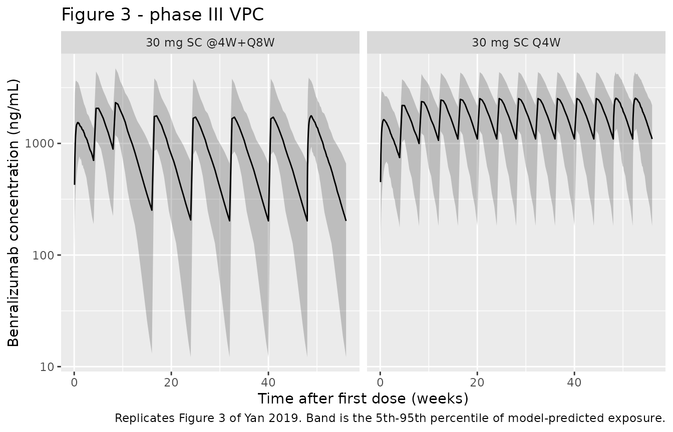
Replicates Figure 3 of Yan 2019: VPC of benralizumab serum concentration under the two phase III regimens.

Yan 2019 publishes no digitised percentile values for Figure 3, so the assertions below test structural features plus an exact steady-state mass balance rather than band widths.

ss_window <- sim |> filter(week >= 40)

trough_by_arm <- ss_window |>
  group_by(arm, id) |>
  summarise(trough = min(Cc_ngml), .groups = "drop") |>
  group_by(arm) |>
  summarise(median_trough = median(trough), .groups = "drop")

trough_by_arm
#> # A tibble: 2 × 2
#>   arm              median_trough
#>   <chr>                    <dbl>
#> 1 30 mg SC @4W+Q8W          202.
#> 2 30 mg SC Q4W             1096.

# Per-patient steady-state mass balance over the final dosing interval:
# cl_i * AUCtau_i == fdepot_i * Dose exactly once steady state is reached.
# Both sides use the SAME drawn parameters, so the only discrepancy is
# trapezoidal integration error and a tight bound is the correct one.
ss_recovery <- sim |>
  mutate(
    window_start = last_dose_time[arm],
    window_end = last_dose_time[arm] + interval_length[arm]
  ) |>
  filter(time >= window_start, time <= window_end) |>
  group_by(arm, id, cl, fdepot) |>
  arrange(time, .by_group = TRUE) |>
  summarise(
    auc_tau = sum(diff(time) * (head(Cc, -1) + tail(Cc, -1)) / 2),
    .groups = "drop"
  ) |>
  mutate(recovery = cl * auc_tau / (fdepot * 30))

summary(ss_recovery$recovery)
#>    Min. 1st Qu.  Median    Mean 3rd Qu.    Max. 
#>  0.9972  0.9998  0.9999  0.9998  0.9999  1.0010

stopifnot(
  # Exposure stays inside the decade range of the published panels. Robust
  # quantiles, not extremes: a single low-clearance patient may sit above the
  # plotted axis maximum without that being a model defect.
  quantile(sim$Cc_ngml[sim$week > 1], 0.95) < 5000,
  quantile(sim$Cc_ngml[sim$week > 1], 0.05) > 1,
  # The same dose given Q4W accumulates to a higher trough than given Q8W.
  trough_by_arm$median_trough[trough_by_arm$arm == "30 mg SC Q4W"] >
    trough_by_arm$median_trough[trough_by_arm$arm == "30 mg SC @4W+Q8W"],
  # Steady-state mass balance holds for every simulated patient.
  all(abs(ss_recovery$recovery - 1) < 0.01)
)

Replicate Figure 4: body weight and ADA effects on clearance

Figure 4 plots individual benralizumab CL against body weight, with closed circles for ADA-negative and open circles for ADA-positive patients, and a red prediction curve the caption prints as CL.(body weight/70)^0.807.

cl_by_subject <- sim |>
  distinct(id, arm, WT, ADA_POS, cl)

curve_df <- tibble::tibble(WT = seq(40, 205, length.out = 200)) |>
  mutate(cl = 0.291 * (WT / 70)^0.807)

ggplot(cl_by_subject, aes(WT, cl)) +
  geom_point(aes(shape = factor(ADA_POS)), alpha = 0.45) +
  geom_line(data = curve_df, colour = "red", linewidth = 1) +
  scale_shape_manual(
    values = c(`0` = 16, `1` = 1),
    labels = c(`0` = "ADA negative", `1` = "ADA positive"),
    name = NULL
  ) +
  labs(
    x = "Body weight (kg)",
    y = "Benralizumab CL (L/day)",
    title = "Figure 4 - body weight and ADA effects on CL",
    caption = "Replicates Figure 4 of Yan 2019. Red line is CL * (body weight / 70)^0.807."
  )

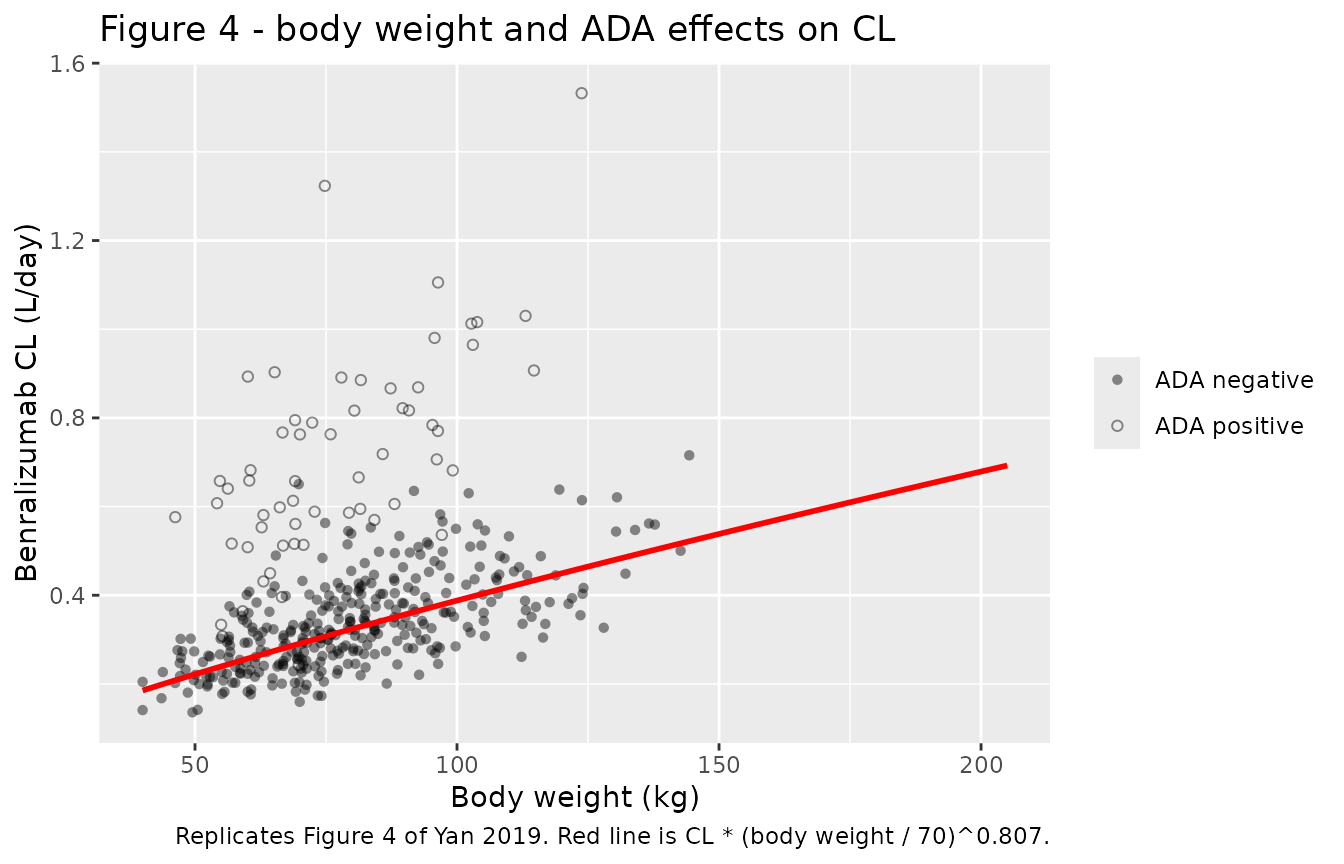
Replicates Figure 4 of Yan 2019: individual clearance versus body weight, split by ADA status.

The scatter in the plot is inter-individual variability on clearance (etalcl, 24.2 %CV), exactly as in the published figure, where the points are individual post-hoc estimates. Two checks are therefore needed: an exact one on the curve itself, and a robust one on the cohort.

# Exact check. With the random effects zeroed, the model's clearance must equal
# CL * (WT/70)^0.807 * 2.24^ADA_POS at every weight and both ADA states. This is
# deterministic, so it is checked to machine precision.
curve_grid <- tidyr::expand_grid(
  WT = c(40, 55, 70, 90, 120, 160, 204.4),
  ADA_POS = c(0, 1)
) |>
  mutate(id = row_number(), STUDY_MICP220 = 0)

curve_events <- bind_rows(
  curve_grid |> mutate(time = 0, amt = 30, evid = 1L, cmt = "depot", dvid = NA_integer_),
  curve_grid |>
    tidyr::expand_grid(time = c(1, 2)) |>
    mutate(amt = NA_real_, evid = 0L, cmt = "central", dvid = 1L)
) |>
  arrange(id, time, desc(evid))

# The "multi-subject simulation without 'omega'" warning is expected and wanted
# here: the solve is deliberately deterministic across several subjects.
curve_check <- suppressWarnings(rxode2::rxSolve(
  mod_typ, curve_events,
  omega = NA, useLinCmt = FALSE,
  keep = c("WT", "ADA_POS"), returnType = "data.frame"
)) |>
  distinct(id, WT, ADA_POS, cl) |>
  mutate(published_curve = 0.291 * (WT / 70)^0.807 * 2.24^ADA_POS)

max(abs(curve_check$cl / curve_check$published_curve - 1))
#> [1] 5.107026e-15

stopifnot(
  nrow(curve_check) == nrow(curve_grid),
  all(abs(curve_check$cl / curve_check$published_curve - 1) < 1e-8)
)

# Robust check on the cohort. Dividing out the weight effect leaves
# exp(etalcl) * 2.24^ADA_POS, whose median is 1 for ADA-negative patients and
# 2.24 for ADA-positive ones. Medians, not extremes -- individual points are
# spread by the 24.2 %CV clearance IIV.
normalised <- cl_by_subject |>
  mutate(cl_norm = cl / (0.291 * (WT / 70)^0.807)) |>
  group_by(`ADA status` = ifelse(ADA_POS == 1, "ADA positive", "ADA negative")) |>
  summarise(n = n(), median_normalised_cl = median(cl_norm), .groups = "drop")

normalised
#> # A tibble: 2 × 3
#>   `ADA status`     n median_normalised_cl
#>   <chr>        <int>                <dbl>
#> 1 ADA negative   341                 1.01
#> 2 ADA positive    59                 2.17

med_neg <- normalised$median_normalised_cl[normalised$`ADA status` == "ADA negative"]
med_pos <- normalised$median_normalised_cl[normalised$`ADA status` == "ADA positive"]

stopifnot(
  all(normalised$n > 10),
  # median(exp(etalcl)) = 1 by construction; the bound covers sampling noise.
  abs(med_neg - 1) < 0.10,
  # ... and the ADA-positive group sits 2.24-fold above it.
  abs(med_pos / 2.24 - 1) < 0.20
)

Yan 2019 Figure 5 is the complementary negative result: benralizumab CL is flat at 0.30-0.31 L/day across strata of estimated GFR and of baseline blood eosinophil count. That figure needs no simulation to reproduce – eGFR and eosinophil count are absent from the final model, so CL is invariant to them by construction. Both are recorded in covariatesDataExcluded with the paper’s reasoning, including why the eosinophil result is mechanistically load-bearing for a cytolytic anti-eosinophil antibody.

Cohort NCA and the terminal half-life

A separate single-dose cohort is used for the cohort-level NCA, because a multiple-dose profile has no clean terminal phase. Both routes are simulated at 30 mg so the AUC ratio recovers the absolute bioavailability under full between-subject variability.

sd_cohort <- bind_rows(
  make_cohort(n_per_arm, "30 mg SC single dose", id_offset = 1000L),
  make_cohort(n_per_arm, "30 mg IV single dose", id_offset = 1000L + n_per_arm)
)

sd_obs_times <- sort(unique(c(seq(0, 28, by = 0.25), seq(28, 180, by = 2))))

sd_doses <- sd_cohort |>
  mutate(
    time = 0, amt = 30, evid = 1L, dvid = NA_integer_,
    cmt = ifelse(arm == "30 mg IV single dose", "central", "depot")
  )

sd_events <- bind_rows(
  sd_doses,
  sd_cohort |>
    tidyr::expand_grid(time = sd_obs_times) |>
    mutate(amt = NA_real_, evid = 0L, cmt = "central", dvid = 1L)
) |>
  arrange(id, time, desc(evid))

rxode2::rxSetSeed(20190312)
sim_sd <- rxode2::rxSolve(
  mod, sd_events,
  keep = c("arm", "WT", "ADA_POS"),
  useLinCmt = FALSE,
  returnType = "data.frame"
)

stopifnot(nrow(sim_sd) > 0, all(is.finite(sim_sd$Cc)))

sim_nca <- sim_sd |>
  filter(!is.na(Cc)) |>
  select(id, time, Cc, treatment = arm)

# Guarantee a time = 0 record per patient. For the subcutaneous arm the
# pre-dose concentration is genuinely zero; for the intravenous arm rxSolve
# already returns the post-bolus value at time 0, which `distinct()` keeps.
sim_nca <- bind_rows(
  sim_nca,
  sim_nca |> distinct(id, treatment) |> mutate(time = 0, Cc = 0)
) |>
  distinct(id, treatment, time, .keep_all = TRUE) |>
  arrange(id, treatment, time)

nca_res <- PKNCA::pk.nca(PKNCA::PKNCAdata(
  PKNCA::PKNCAconc(sim_nca, Cc ~ time | treatment + id),
  PKNCA::PKNCAdose(sd_doses |> select(id, time, amt, treatment = arm),
    amt ~ time | treatment + id
  ),
  intervals = data.frame(
    start = 0, end = Inf,
    cmax = TRUE, tmax = TRUE, aucinf.obs = TRUE, half.life = TRUE
  )
))

nca_df <- as.data.frame(nca_res)

nca_df |>
  filter(PPTESTCD %in% c("cmax", "tmax", "aucinf.obs", "half.life")) |>
  group_by(treatment, PPTESTCD) |>
  summarise(median = median(PPORRES, na.rm = TRUE), .groups = "drop") |>
  tidyr::pivot_wider(names_from = PPTESTCD, values_from = median) |>
  rename(
    "Treatment" = treatment,
    "Cmax (mg/L)" = cmax,
    "Tmax (day)" = tmax,
    "AUC0-inf (mg*day/L)" = aucinf.obs,
    "t1/2 (day)" = half.life
  ) |>
  knitr::kable(digits = 3, caption = "Median simulated NCA parameters over the cohort.")

Median simulated NCA parameters over the cohort.
Treatment	AUC0-inf (mg*day/L)	Cmax (mg/L)	t1/2 (day)	Tmax (day)
30 mg IV single dose	90.677	9.089	12.481	0.000
30 mg SC single dose	51.346	1.687	14.179	6.375

# Per-patient mass balance from PKNCA's AUCinf on the subcutaneous arm. Same
# drawn parameters on both sides, so this stays tight.
sc_recovery <- nca_df |>
  filter(PPTESTCD == "aucinf.obs") |>
  inner_join(sim_sd |> distinct(id, arm, cl, fdepot), by = c("id", "treatment" = "arm")) |>
  filter(treatment == "30 mg SC single dose") |>
  mutate(recovery = cl * PPORRES / (fdepot * 30))

auc_median <- nca_df |>
  filter(PPTESTCD == "aucinf.obs") |>
  group_by(treatment) |>
  summarise(median_auc = median(PPORRES, na.rm = TRUE), .groups = "drop")

f_recovered <- auc_median$median_auc[auc_median$treatment == "30 mg SC single dose"] /
  auc_median$median_auc[auc_median$treatment == "30 mg IV single dose"]

c(
  median_sc_mass_balance = median(sc_recovery$recovery),
  f_recovered = f_recovered,
  f_published = 0.589
)
#> median_sc_mass_balance            f_recovered            f_published 
#>              0.9998734              0.5662514              0.5890000

stopifnot(
  nrow(sc_recovery) == n_per_arm,
  abs(median(sc_recovery$recovery) - 1) < 0.005,
  quantile(abs(sc_recovery$recovery - 1), 0.95) < 0.02,
  # The two arms are different patients with independently drawn etas, so the
  # ratio of their median AUCs is a cohort statistic and carries sampling
  # noise; a loose relative bound is the honest one here.
  abs(f_recovered / 0.589 - 1) < 0.12
)

Where the published 15.5 days sits

individual_half_life <- sim_sd |>
  distinct(id, arm, ADA_POS, cl, vc, q, vp) |>
  mutate(t_half = terminal_half_life(cl, vc, q, vp))

hl_summary <- individual_half_life |>
  group_by(`ADA status` = ifelse(ADA_POS == 1, "ADA positive", "ADA negative")) |>
  summarise(
    n = n(),
    `median t1/2 (day)` = median(t_half),
    `mean t1/2 (day)` = mean(t_half),
    .groups = "drop"
  )

hl_summary |>
  knitr::kable(digits = 2, caption = "Individual terminal half-life by ADA status.")

Individual terminal half-life by ADA status.
ADA status	n	median t1/2 (day)	mean t1/2 (day)
ADA negative	331	14.33	15.66
ADA positive	69	7.79	8.32


c(
  typical_value_ada_negative = t_half_terminal,
  published = 15.5
)
#> typical_value_ada_negative                  published 
#>                   14.61769                   15.50000

Three facts, in order of how much they matter:

Anti-drug antibodies raise CL 2.24-fold, which roughly halves the terminal half-life for the 15.62% of patients who develop them. The cohort split above shows the two groups separately.
Within the ADA-negative group the terminal half-life is right-skewed – the mean sits above the median, and both sit above the 70 kg typical-value computation of 14.62 days. The published 15.5 days falls inside that ADA-negative range.
The Discussion reports the same statistic stratified by age: “median estimates of approximately 14 days in adolescents, 15 days in adults (18-64 years of age), and 17 days in older adults”. A single “approximately 15.5 days” summarising that spread is consistent with what the model produces; it is not the typical-subject value.

ada_neg_hl <- individual_half_life$t_half[individual_half_life$ADA_POS == 0]
ada_pos_hl <- individual_half_life$t_half[individual_half_life$ADA_POS == 1]

stopifnot(
  length(ada_neg_hl) > 50, length(ada_pos_hl) > 10,
  # ADA positivity shortens the terminal half-life (2.24-fold higher CL).
  median(ada_neg_hl) > median(ada_pos_hl),
  # The distribution is right-skewed, so the mean exceeds the median.
  mean(ada_neg_hl) > median(ada_neg_hl),
  # The published 15.5 days is within 25% of the ADA-negative cohort median.
  # Centre, not extreme, and loose enough to survive a different random draw.
  abs(median(ada_neg_hl) / 15.5 - 1) < 0.25,
  # The deterministic closed form is pinned exactly.
  abs(t_half_terminal - 14.62) < 0.05
)

Assumptions and deviations

No published NCA table. Yan 2019 reports model parameters, VPC figures and covariate-effect figures, but no Cmax / Tmax / AUC table. The comparison table above therefore has a single reference value, the terminal half-life, and the weight of the validation rests on the closed-form structural checks, the steady-state mass balance and the figure replications.
The MI-CP220 bioavailability row is read as an absolute fraction. Table 5 labels it “Change in F with study CP220, fraction”, the same wording as the ADA row directly above it where the number is a multiplier. The reasoning for reading this one differently is set out in full under “Two table-reading decisions worth recording”, and rests on the ratio agreement with the independent Jin 2025 refit plus the stratum’s own separately tabulated IIV. This is the single interpretive decision in the extraction that a reviewer should check first.
IIV percentages are read as 100 * omega_SD. Pinned by the IIV(Q) value that Table 4 states as a variance and Table 5 prints as a percentage. Note that the successor paper Jin 2025 uses the other convention (the exact lognormal CV) for the same quantity, so the two tables cannot be compared percentage-to-percentage.
Residual error is encoded as lnorm(). Yan 2019 Equation 2 writes a combined proportional-plus-additive error, but Results 3.2 states the data were log-transformed and a log-normal residual error used, and Table 5 reports only proportional components. Additive error on log-concentration is exactly lnorm(). The additive component of Equation 2 has no published estimate and is not carried.
No body weight effect on Q. Table 5 lists “Body weight on Q, power” as 0 with no confidence interval, i.e. the Wald’s Approximation Method step dropped it. No zero-valued exponent is encoded; Q simply carries no covariate.
Intravenous doses are simulated as bolus injections. The phase I/II studies administered benralizumab by intravenous infusion, but Yan 2019 does not report infusion durations and the model carries no dur() term. AUCinf is independent of infusion duration, so the bioavailability and half-life checks are unaffected; the simulated intravenous Cmax is an upper bound and is not compared against anything published.
Covariate distributions are assumed. Body weight is drawn lognormal with the median and mean/median ratio of Yan 2019 Table 2 and truncated to the observed range; ADA status is drawn Bernoulli at the pooled 15.62% rate of Table 3 and held constant per patient, whereas the source dataset assessed it at each visit and therefore carried it as time-varying. The published race, sex and age distributions are recorded in the model’s population metadata but are not simulated, because none of them entered the final model.
The VPC band is model-predicted exposure without residual error. Cc from rxSolve() is the individual prediction; the published Figure 3 bands are prediction intervals that include the study-stratified residual error. The simulated band is therefore narrower than the published one, which is why the Figure 3 assertions test structural features rather than band widths.
Typographical error in the source. Yan 2019 Tables 2 and 3 print “NCT00768079” twice in their column headers. The fourth column (n = 19) is NCT00783289, the fifth study named in Table 1 and in Results 3.2. This affects only the demographic tables, not any model parameter.
No supplement and no erratum. EuropePMC records no supplementary files and no correction notice for PMC6584252, and the article text references neither. Every value used here comes from the main text and its tables.