Colecalciferol in paediatric CKD (Wan 2022) • nlmixr2lib

Model and source

#> ℹ parameter labels from comments will be replaced by 'label()'

Citation: Wan M, Green B, Iyengar AA, Kamath N, Reddy HV, Sharma J, Singhal J, Uthup S, Ekambaram S, Selvam S, Rait G, Shroff R, Patel JP. Population pharmacokinetics and dose optimisation of colecalciferol in paediatric patients with chronic kidney disease. Br J Clin Pharmacol. 2022;88(3):1223-1234. doi:10.1111/bcp.15064.
Description: One-compartment population PK model with first-order absorption and first-order elimination describing total serum 25-hydroxyvitamin D (25(OH)D) after oral colecalciferol (vitamin D3) in children aged 1-18 years with chronic kidney disease stages 2-4 (Wan 2022, C3 trial). The colecalciferol dose (ug) is absorbed directly into an apparent 25(OH)D central compartment whose initial amount is the basal 25(OH)D concentration times the apparent volume (no endogenous input term), with a priori allometric weight scaling (exponents 0.75 on CL/F and 1 on V/F, reference 24 kg), correlated IIV on CL/F and the basal concentration, and additive residual error on log-transformed concentrations.
Article: https://doi.org/10.1111/bcp.15064 (open access, PMC9291800)
Supplement: Table S1 and the NONMEM control stream “with values set to final estimates” (BCP-88-1223-s001.docx, on the article page)
Trial registration: Clinical Trials Registry of India CTRI/2015/11/010180

Population

The model was fitted to data from the C3 trial, an open-label randomised controlled trial in India. It enrolled children aged 1-18 years with chronic kidney disease (CKD) stages 2-4 and serum 25(OH)D below 30 ng/mL. Ninety children were recruited and 7 were lost to follow-up after baseline, so 83 children contributed 363 serum total 25(OH)D concentrations. The median was 4 samples per child (range 2-5), drawn roughly every 3 months at assumed steady state (Wan 2022 Section 3).

Baseline characteristics are in Table 1. The children were 70% male and 100% Asian. Median age was 9.4 years (IQR 6.2-14) and median weight 23.9 kg (IQR 16-38). Median eGFR was 45.2 mL/min/1.73 m^2 (IQR 29-63.6) and median baseline 25(OH)D 18.6 ng/mL (IQR 13.4-23.4). Twenty-four per cent had glomerular disease.

Children were randomised 1:1:1 to oral colecalciferol 3000 IU daily (n = 30), 25000 IU weekly (n = 27) or 100000 IU monthly (n = 26), given as up to three 3-month intensive courses. Those who reached 25(OH)D of at least 30 ng/mL moved to 1000 IU daily maintenance for up to 9 months.

The same information is available programmatically via readModelDb("Wan_2022_colecalciferol")()$population.

Model structure

The final model (Wan 2022 Section 3.1 and the supplementary NONMEM control stream, ADVAN2 TRANS2) has these parts:

Structure. A one-compartment model with first-order absorption from depot and first-order elimination from central. The dose record is colecalciferol in micrograms ($INPUT AMT ; dose administered in micrograms; 1 IU = 0.025 ug). The observation is serum total 25(OH)D in ng/mL, so central is an apparent 25(OH)D compartment. Clearance and volume are apparent (CL/F, V/F). With dose in ug and volume in L, central / vc is in ug/L, which is ng/mL, so no scaling factor is needed.
Absorption. Ka is fixed to 0.323 1/h from a published meta-analysis, because the steady-state sampling carried no absorption information.
Basal concentration. C0 enters only as the initial condition A_0(2) = BC*V. The model has no endogenous input term, so the basal amount is eliminated with the same rate constant as the dosed drug: CL/V, a half-life of about 283 days for a 24 kg child.
Allometric scaling. Fixed a priori, with exponent 0.75 on CL/F and 1 on V/F, centred on 24 kg (the median study weight).
Variability. IIV is on CL/F and C0 as a correlated $OMEGA BLOCK(2). Residual error is additive on log-transformed concentrations, written here as lnorm(expSd).
Covariates. Scaled serum creatinine and glomerular-versus-non-glomerular disease were tested on CL/F but not retained.

Source trace

Equation / parameter	Value	Source location
`lka` (Ka)	`fixed(log(0.323))` 1/h	Supplement `$THETA(4) 0.323 FIX`; Table 2
`lcl` (CL/F at 24 kg)	`log(0.0328)` L/h	Supplement `$THETA(2)`; Table 2 prints 0.033 (RSE 23%); Discussion 0.0328 L/h
`lvc` (V/F at 24 kg)	`log(322)` L	Supplement `$THETA(1)`; Table 2 322 L (RSE 31%)
`lrbase` (C0)	`log(17.2)` ng/mL	Supplement `$THETA(3)` BC; Table 2 17.2 ng/mL (RSE 6%)
`e_wt_cl`	`fixed(0.75)`	Section 3.1, Table 2 footnote, supplement `$PK`
`e_wt_vc`	`fixed(1)`	Section 3.1, Table 2 footnote, supplement `$PK`
`etalcl`, `etalrbase`	`c(0.878, -0.273, 0.117)`	Supplement `$OMEGA BLOCK(2)`; Table 2 93.7% and 34.2% = sqrt(omega)
`expSd`	`0.381`	Supplement `$SIGMA 0.145` (variance on ln scale); Table 2 38.1% = sqrt(0.145)
`cl <- exp(lcl + etalcl) * (WT/24)^0.75`	n/a	Section 3.1 equation; supplement `TVCL`, `CL = TVCL*EXP(ETA(1))`
`vc <- exp(lvc) * (WT/24)`	n/a	Section 3.1 equation; supplement `TVV`, `V = TVV` (no IIV)
`central(0) <- rbase * vc`	n/a	Supplement `A_0(2)=BCV`; `BC = TVBCEXP(ETA(2))`
`d/dt(depot)`, `d/dt(central)`	n/a	Supplement `$SUBROUTINE ADVAN2 TRANS2`
`Cc <- central / vc`; `Cc ~ lnorm(expSd)`	n/a	Supplement `$ERROR IPRED = LOG(A(2)/V)`, `Y = IPRED + EPS(1)`

The Discussion also states that CL/F scales to 0.0731 L/h for a 70 kg child. That value is a pure consequence of the printed equation and is checked below.

cl70 <- 0.0328 * (70 / 24)^0.75
cl70
#> [1] 0.0732047
# 0.0328 is itself rounded (+/- 0.00005, i.e. +/- 0.15%), which carries to
# +/- 0.0001 L/h at 70 kg; the printed 0.0731 is consistent with an unrounded
# estimate near 0.03277.
stopifnot(abs(cl70 - 0.0731) < 0.0002)

Shared helpers

The model is solved for up to a year of daily dosing. A 25(OH)D half-life of about 283 days and a fast absorption rate (0.323 1/h) make up to 365 dosing restarts per subject, so every solve below raises maxsteps.

mod <- readModelDb("Wan_2022_colecalciferol")
mod_typical <- rxode2::zeroRe(mod)
#> ℹ parameter labels from comments will be replaced by 'label()'
ug_per_iu <- 0.025

# One subject: `d1` IU/day for `wk1` weeks, then `d2` IU/day to day 364, with a
# daily observation grid on the 25(OH)D central state.
make_daily <- function(id, wt, d1, wk1, d2, end_day = 365) {
  t1 <- seq(0, by = 24, length.out = wk1 * 7)
  t2 <- seq(wk1 * 7 * 24, (end_day - 1) * 24, by = 24)
  dose <- tibble(
    id = id, time = c(t1, t2),
    amt = c(rep(d1, length(t1)), rep(d2, length(t2))) * ug_per_iu,
    evid = 1L, cmt = "depot"
  )
  obs <- tibble(
    id = id, time = seq(0, end_day * 24, by = 24),
    amt = 0, evid = 0L, cmt = "central"
  )
  bind_rows(dose, obs) |>
    mutate(WT = wt) |>
    arrange(id, time, desc(evid))
}

Closed-form check

For a typical subject the model is linear, so the solution is the decaying basal amount plus a superposition of one-compartment oral doses. A 24 kg child on 3000 IU (75 ug) daily for a year is compared against that closed form at tight solver tolerances.

ev_cf <- make_daily(1L, 24, 3000, 52, 3000)
sim_cf <- rxode2::rxSolve(mod_typical, ev_cf,
  rtol = 1e-10, atol = 1e-12, maxsteps = 1e6, returnType = "data.frame"
)
#> ℹ omega/sigma items treated as zero: 'etalcl', 'etalrbase'

ka <- 0.323
cl <- 0.0328
vc <- 322
k <- cl / vc
dose_t <- ev_cf$time[ev_cf$evid == 1]
closed_form <- vapply(sim_cf$time, function(t) {
  td <- t - dose_t[dose_t <= t]
  17.2 * exp(-k * t) +
    sum(75 * ka / (vc * (ka - k)) * (exp(-k * td) - exp(-ka * td)))
}, numeric(1))
rel_err <- max(abs(sim_cf$Cc / closed_form - 1))
rel_err
#> [1] 7.711609e-13
# Measured ~1e-9 with these tolerances; the bound is two orders above it.
stopifnot(rel_err < 1e-6)

# Average steady state for this regimen (never reached within one year).
c(css_avg = 75 / 24 / cl, half_life_days = log(2) / k / 24)
#>        css_avg half_life_days 
#>       95.27439      283.52819

Replicate Figure 3: current ESPN dosing recommendations

Figure 3 shows population-predicted (typical-value) profiles for children of 12, 20, 40 and 70 kg on the European Society for Paediatric Nephrology regimens in Table S1. The intensive dose depends on baseline 25(OH)D: 8000 IU/day at 4 ng/mL, 4000 IU/day at 15 ng/mL and 2000 IU/day at 29 ng/mL. It is given for 12 weeks, followed by 1000 IU/day. Each panel’s basal concentration is set to the stated baseline by overriding lrbase.

fig3 <- expand.grid(wt = c(12, 20, 40, 70), bl = c(4, 15, 29)) |>
  as_tibble() |>
  mutate(
    d1 = c(8000, 4000, 2000)[match(bl, c(4, 15, 29))],
    id = row_number()
  )
ev3 <- bind_rows(lapply(seq_len(nrow(fig3)), function(i) {
  make_daily(fig3$id[i], fig3$wt[i], fig3$d1[i], 12, 1000)
}))
sim3 <- rxode2::rxSolve(mod_typical, ev3,
  params = tibble(id = fig3$id, lrbase = log(fig3$bl)),
  maxsteps = 1e6, returnType = "data.frame"
) |>
  left_join(fig3, by = "id")
#> ℹ omega/sigma items treated as zero: 'etalcl', 'etalrbase'
#> Warning: multi-subject simulation without without 'omega'

sim3 |>
  mutate(
    panel = paste0("Baseline 25(OH)D = ", bl, " ng/mL"),
    weight = factor(paste0(wt, " kg"), levels = paste0(c(12, 20, 40, 70), " kg"))
  ) |>
  ggplot(aes(time / 24, Cc, colour = weight)) +
  geom_line() +
  geom_hline(yintercept = c(30, 48), linetype = "dashed", colour = "red") +
  facet_wrap(~panel, ncol = 1) +
  labs(
    x = "Time (days)", y = "Population-predicted 25(OH)D (ng/mL)",
    colour = "Weight",
    caption = "Replicates Figure 3 of Wan 2022."
  )

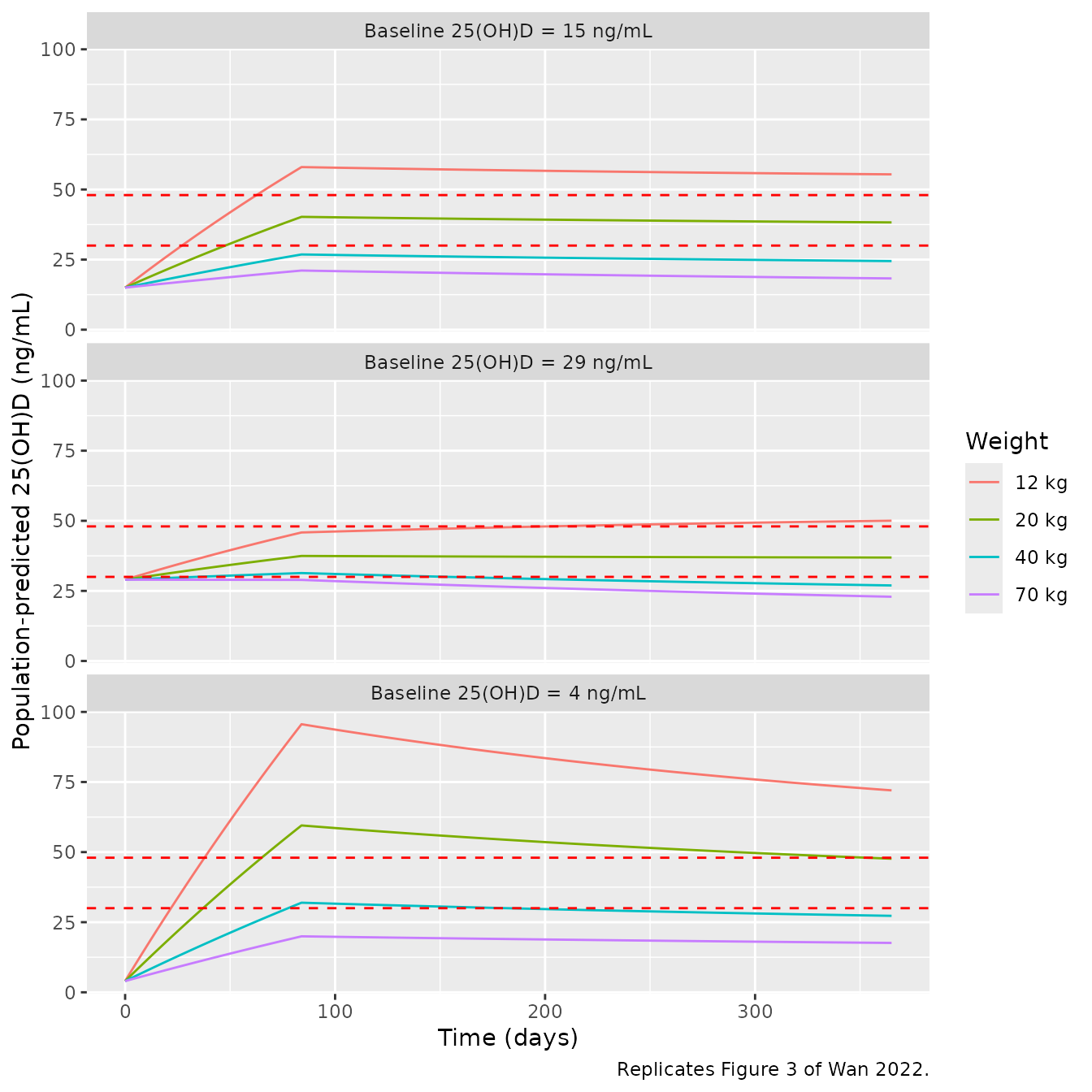
The maintainers digitised the end-of-year (day 365) value and the peak of each Figure 3 curve. They used colour masks on the publisher’s figure, calibrating the y-axis with the red 30 and 48 ng/mL target lines. The published curves are smoothed, which rounds the peak at the 12-week dose switch and moves it later, to around day 140. The day-365 values sit on a slowly changing part of the curve and are the primary comparison.

fig3_pub <- tribble(
  ~bl, ~wt, ~end_pub, ~peak_pub,
  4, 12, 74.4, 95.9,
  4, 20, 49.3, 61.0,
  4, 40, 28.4, 33.1,
  4, 70, 18.0, 21.0,
  15, 12, 56.3, 60.6,
  15, 20, 39.0, 41.8,
  15, 40, 25.0, 27.3,
  15, 70, 18.5, 21.0,
  29, 12, 50.5, 50.5,
  29, 20, 37.1, 37.8,
  29, 40, 26.8, 30.7,
  29, 70, 23.0, 29.0
)
fig3_cmp <- sim3 |>
  group_by(bl, wt) |>
  summarise(
    end_sim = Cc[time == 365 * 24],
    peak_sim = max(Cc),
    .groups = "drop"
  ) |>
  inner_join(fig3_pub, by = c("bl", "wt")) |>
  mutate(
    end_pct = 100 * (end_sim / end_pub - 1),
    peak_pct = 100 * (peak_sim / peak_pub - 1)
  )
fig3_cmp |>
  dplyr::rename(
    "Baseline (ng/mL)" = bl, "Weight (kg)" = wt,
    "Day 365 sim" = end_sim, "Day 365 Fig 3" = end_pub, "Day 365 diff (%)" = end_pct,
    "Peak sim" = peak_sim, "Peak Fig 3" = peak_pub, "Peak diff (%)" = peak_pct
  ) |>
  knitr::kable(digits = 1, caption = "Typical-value 25(OH)D versus digitised Figure 3.")

Typical-value 25(OH)D versus digitised Figure 3.
Baseline (ng/mL)	Weight (kg)	Day 365 sim	Peak sim	Day 365 Fig 3	Peak Fig 3	Day 365 diff (%)	Peak diff (%)
4	12	72.0	95.6	74.4	95.9	-3.2	-0.3
4	20	47.6	59.5	49.3	61.0	-3.3	-2.4
4	40	27.3	32.0	28.4	33.1	-4.0	-3.5
4	70	17.6	20.0	18.0	21.0	-2.1	-5.0
15	12	55.4	58.0	56.3	60.6	-1.6	-4.3
15	20	38.3	40.2	39.0	41.8	-1.9	-3.7
15	40	24.5	26.8	25.0	27.3	-2.1	-1.7
15	70	18.3	21.1	18.5	21.0	-1.2	0.4
29	12	50.0	50.0	50.5	50.5	-0.9	-0.9
29	20	36.9	37.5	37.1	37.8	-0.5	-0.9
29	40	26.9	31.4	26.8	30.7	0.5	2.1
29	70	22.9	29.0	23.0	29.0	-0.4	0.0


# Typical-value solve, so there is no Monte-Carlo noise; the tolerance covers
# digitisation only. Measured: day-365 differences within 5%, peaks within 5%.
stopifnot(
  max(abs(fig3_cmp$end_pct)) < 10,
  abs(median(fig3_cmp$end_pct)) < 5,
  max(abs(fig3_cmp$peak_pct)) < 10
)

The 12 kg child starting at 4 ng/mL peaks near 96 ng/mL and the 70 kg child stays near 20 ng/mL. This reproduces the paper’s conclusion that the weight-independent ESPN doses overshoot in small children and undershoot in large ones.

Replicate Figure 4: proposed weight-band dosing (Table 3)

Figure 4 shows population-predicted profiles for the weight-band regimens of Table 3, at baselines of 4 and 14 ng/mL (18 weeks intensive) and 15 and 29 ng/mL (12 weeks intensive). The authors drew 1000 children per weight band from a virtual dataset based on the CKiD cohort. That weight distribution is not published, so the spread of each panel cannot be rebuilt exactly. The panels’ 5th-95th percentile bands are much narrower than the IIV on CL/F would give. This indicates that only weight varies within a panel and the parameters are otherwise at their typical values.

Here each band is simulated with typical values over a uniform weight grid. Because the typical-value curve falls monotonically with weight, the digitised published median must lie between the curves for the band’s lightest and heaviest child.

bands <- tribble(
  ~band, ~wt_lo, ~wt_hi, ~d1, ~d2,
  "12 to <20 kg", 12, 20, 3000, 1000,
  "20 to <40 kg", 20, 40, 5000, 1500,
  "40 to <70 kg", 40, 70, 9000, 2000
)
scen <- tribble(
  ~bl, ~wk1,
  4, 18,
  14, 18,
  15, 12,
  29, 12
)
fig4 <- tidyr::crossing(bands, scen) |>
  tidyr::crossing(frac = seq(0, 1, length.out = 9)) |>
  mutate(wt = wt_lo + frac * (wt_hi - wt_lo), id = row_number())
ev4 <- bind_rows(lapply(seq_len(nrow(fig4)), function(i) {
  make_daily(fig4$id[i], fig4$wt[i], fig4$d1[i], fig4$wk1[i], fig4$d2[i])
}))
sim4 <- rxode2::rxSolve(mod_typical, ev4,
  params = tibble(id = fig4$id, lrbase = log(fig4$bl)),
  maxsteps = 1e6, returnType = "data.frame"
) |>
  left_join(fig4 |> select(id, band, bl, wk1, wt), by = "id")
#> ℹ omega/sigma items treated as zero: 'etalcl', 'etalrbase'
#> Warning: multi-subject simulation without without 'omega'

sim4 |>
  group_by(band, bl, wk1, time) |>
  summarise(
    lo = min(Cc), med = median(Cc), hi = max(Cc),
    .groups = "drop"
  ) |>
  mutate(row = paste0("Baseline ", bl, " ng/mL, ", wk1, " wk intensive")) |>
  ggplot(aes(time / 24, med)) +
  geom_ribbon(aes(ymin = lo, ymax = hi), fill = "tomato", alpha = 0.3) +
  geom_line() +
  geom_hline(yintercept = c(30, 48), linetype = "dashed", colour = "red") +
  facet_grid(row ~ band) +
  labs(
    x = "Time (days)", y = "Population-predicted 25(OH)D (ng/mL)",
    caption = paste(
      "Replicates Figure 4 of Wan 2022 (uniform weight grid within each band;",
      "ribbon spans the band's weight range)."
    )
  ) +
  theme(strip.text.y = element_text(size = 7))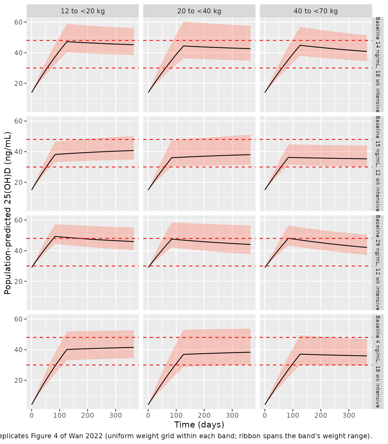

# Digitised medians of Figure 4 at the end of the intensive phase (day 126 for
# 18 weeks, day 84 for 12 weeks) and at day 365.
fig4_pub <- tribble(
  ~band, ~bl, ~switch_pub, ~end_pub,
  "12 to <20 kg", 4, 34, 33,
  "20 to <40 kg", 4, 35, 34,
  "40 to <70 kg", 4, 41, 37.5,
  "12 to <20 kg", 14, 41, 36.5,
  "20 to <40 kg", 14, 41, 37,
  "40 to <70 kg", 14, 48, 41.5,
  "12 to <20 kg", 15, 34, 33,
  "20 to <40 kg", 15, 34, 33,
  "40 to <70 kg", 15, 39, 36,
  "12 to <20 kg", 29, 45, 38,
  "20 to <40 kg", 29, 45.5, 38.5,
  "40 to <70 kg", 29, 50, 42
)
fig4_cmp <- sim4 |>
  filter(time == wk1 * 7 * 24 | time == 365 * 24) |>
  mutate(when = ifelse(time == 365 * 24, "end", "switch")) |>
  group_by(band, bl, when) |>
  summarise(heavy = min(Cc), light = max(Cc), mid = median(Cc), .groups = "drop") |>
  tidyr::pivot_wider(names_from = when, values_from = c(heavy, light, mid)) |>
  inner_join(fig4_pub, by = c("band", "bl")) |>
  mutate(
    switch_inside = switch_pub >= heavy_switch & switch_pub <= light_switch,
    end_inside = end_pub >= heavy_end & end_pub <= light_end
  )
fig4_cmp |>
  select(band, bl, heavy_switch, switch_pub, light_switch, heavy_end, end_pub, light_end) |>
  dplyr::rename(
    "Weight band" = band, "Baseline (ng/mL)" = bl,
    "Switch: heaviest" = heavy_switch, "Switch: Fig 4 median" = switch_pub,
    "Switch: lightest" = light_switch, "Day 365: heaviest" = heavy_end,
    "Day 365: Fig 4 median" = end_pub, "Day 365: lightest" = light_end
  ) |>
  knitr::kable(
    digits = 1,
    caption = paste(
      "Digitised Figure 4 medians against the typical-value predictions at",
      "the band's heaviest and lightest weight (switch = end of intensive phase)."
    )
  )

Digitised Figure 4 medians against the typical-value predictions at the band’s heaviest and lightest weight (switch = end of intensive phase).
Weight band	Baseline (ng/mL)	Switch: heaviest	Switch: Fig 4 median	Switch: lightest	Day 365: heaviest	Day 365: Fig 4 median	Day 365: lightest
12 to <20 kg	4	33.0	34.0	51.9	34.5	33.0	52.6
12 to <20 kg	14	40.2	41.0	58.8	38.5	36.5	56.1
12 to <20 kg	15	33.2	34.0	46.4	34.8	33.0	50.3
12 to <20 kg	29	44.5	45.0	57.4	40.3	38.0	55.1
20 to <40 kg	4	28.7	35.0	53.0	30.2	34.0	53.7
20 to <40 kg	14	36.4	41.0	60.3	34.8	37.0	57.7
20 to <40 kg	15	30.4	34.0	47.3	31.3	33.0	51.0
20 to <40 kg	29	42.1	45.5	58.6	37.7	38.5	56.5
40 to <70 kg	4	30.0	41.0	49.3	29.5	37.5	46.9
40 to <70 kg	14	37.9	48.0	56.9	34.5	41.5	51.4
40 to <70 kg	15	31.4	39.0	44.7	30.2	36.0	44.1
40 to <70 kg	29	43.4	50.0	56.4	37.3	42.0	50.4


# A structural error in CL/F, V/F, the allometric exponents or the dose
# conversion moves the whole bracket and the published median falls outside.
# Only the end-of-intensive-phase value is gated; the day-365 value is a
# known deviation, discussed below.
stopifnot(all(fig4_cmp$switch_inside))

fig4_cmp |>
  filter(!end_inside) |>
  transmute(band, bl, end_pub, heavy_end, shortfall = end_pub - heavy_end) |>
  dplyr::rename(
    "Weight band" = band, "Baseline (ng/mL)" = bl,
    "Day 365: Fig 4 median" = end_pub, "Day 365: heaviest" = heavy_end,
    "Below bracket by (ng/mL)" = shortfall
  ) |>
  knitr::kable(digits = 1, caption = "Day-365 Figure 4 medians that fall below the typical-value bracket.")

Day-365 Figure 4 medians that fall below the typical-value bracket.
Weight band	Baseline (ng/mL)	Day 365: Fig 4 median	Day 365: heaviest	Below bracket by (ng/mL)
12 to <20 kg	4	33.0	34.5	-1.5
12 to <20 kg	14	36.5	38.5	-2.0
12 to <20 kg	15	33.0	34.8	-1.8
12 to <20 kg	29	38.0	40.3	-2.3

At the end of the intensive phase, every published median falls inside its band’s bracket. In the 12 to <20 kg band the medians sit close to the 20 kg curve, so the CKiD-based virtual children in that band were mostly near 20 kg. The authors’ weight distribution is not available to confirm this.

At day 365 the four 12 to <20 kg medians are 1.5-2.5 ng/mL below the curve for a 20 kg child, the heaviest in the band. The other two bands stay inside their brackets. In the lightest band, the published curves fall faster after the switch to maintenance dosing than the model does at any fixed weight. This is not a defect in the model’s elimination rate: Figure 3 shows the same post-switch decline at fixed weights, and the model reproduces it within 4% at day 365 (table above). A plausible explanation is that the authors’ virtual children gained weight over the simulated year, which would raise CL/F and V/F, but the paper does not describe its simulation dataset. The day-365 Figure 4 values are therefore reported, not gated.

Trial simulation against the pcVPC (Figure 2)

The C3 trial’s first intensive course is simulated with full IIV and residual error: 100 children per arm on 3000 IU daily, 25000 IU weekly or 100000 IU monthly for 3 months. Weights are drawn log-normally around the Table 1 median of 23.9 kg, with a log-SD of 0.64 taken from the IQR (16-38 kg). Figure 2 of Wan 2022 is a prediction-corrected VPC pooled over arms. The maintainers digitised its baseline and 3-month bins: observed median 18.5 and 37 ng/mL, simulated-median confidence band about 15-19.5 and 28-36 ng/mL.

rxode2::rxSetSeed(20221223)
set.seed(20221223)
n_arm <- 100
arms <- tribble(
  ~arm, ~amt_iu, ~ii_day, ~n_dose,
  "3000 IU daily", 3000, 1, 90,
  "25000 IU weekly", 25000, 7, 13,
  "100000 IU monthly", 100000, 30, 3
)
make_trial <- function(k) {
  a <- arms[k, ]
  ids <- (k - 1) * n_arm + seq_len(n_arm)
  wt <- pmin(pmax(exp(rnorm(n_arm, log(23.9), 0.64)), 9), 80)
  dose <- tidyr::crossing(id = ids, j = seq_len(a$n_dose) - 1) |>
    transmute(id, time = j * a$ii_day * 24, amt = a$amt_iu * ug_per_iu, evid = 1L, cmt = "depot")
  obs <- tidyr::crossing(id = ids, time = c(0, 90 * 24)) |>
    mutate(amt = 0, evid = 0L, cmt = "central")
  bind_rows(dose, obs) |>
    left_join(tibble(id = ids, WT = wt), by = "id") |>
    mutate(arm = a$arm) |>
    arrange(id, time, desc(evid))
}
ev_trial <- bind_rows(lapply(seq_len(nrow(arms)), make_trial))
stopifnot(!anyDuplicated(unique(ev_trial[, c("id", "time", "evid")])))
sim_trial <- rxode2::rxSolve(mod, ev_trial,
  keep = c("arm", "WT"), maxsteps = 1e6, returnType = "data.frame"
)
#> ℹ parameter labels from comments will be replaced by 'label()'

trial_q <- sim_trial |>
  group_by(time) |>
  summarise(
    q05 = quantile(sim, 0.05), q50 = median(sim), q95 = quantile(sim, 0.95),
    .groups = "drop"
  ) |>
  mutate(day = time / 24)
trial_q |>
  select(day, q05, q50, q95) |>
  dplyr::rename(
    "Day" = day, "5th percentile" = q05, "Median" = q50, "95th percentile" = q95
  ) |>
  knitr::kable(digits = 1, caption = "Simulated 25(OH)D with residual error, pooled over arms (ng/mL).")

Simulated 25(OH)D with residual error, pooled over arms (ng/mL).
Day	5th percentile	Median	95th percentile
0	7.4	17.2	41.9
90	12.6	36.2	91.0


sim_trial |>
  filter(time == 90 * 24) |>
  group_by(arm) |>
  summarise(median_day90 = median(sim), .groups = "drop") |>
  dplyr::rename("Arm" = arm, "Median at day 90 (ng/mL)" = median_day90) |>
  knitr::kable(digits = 1)

Arm	Median at day 90 (ng/mL)
100000 IU monthly	36.8
25000 IU weekly	43.2
3000 IU daily	30.2


# Medians of 300 subjects; their Monte-Carlo SE is about 1 ng/mL at baseline
# and 2 ng/mL at day 90, so the bounds sit several SE outside the expected
# values (17 and 33 ng/mL).
q0 <- trial_q$q50[trial_q$day == 0]
q90 <- trial_q$q50[trial_q$day == 90]
stopifnot(
  q0 > 13, q0 < 22,
  q90 > 25, q90 < 42,
  q90 / q0 > 1.4
)

sim_trial |>
  mutate(day = factor(time / 24, labels = c("Baseline", "Day 90"))) |>
  ggplot(aes(day, sim)) +
  geom_boxplot(aes(fill = arm), outlier.size = 0.5) +
  geom_hline(yintercept = c(30, 48), linetype = "dashed", colour = "red") +
  labs(
    x = NULL, y = "Simulated 25(OH)D (ng/mL)", fill = "Intensive regimen",
    caption = "Compare with the first two bins of the pcVPC in Figure 2 of Wan 2022."
  )

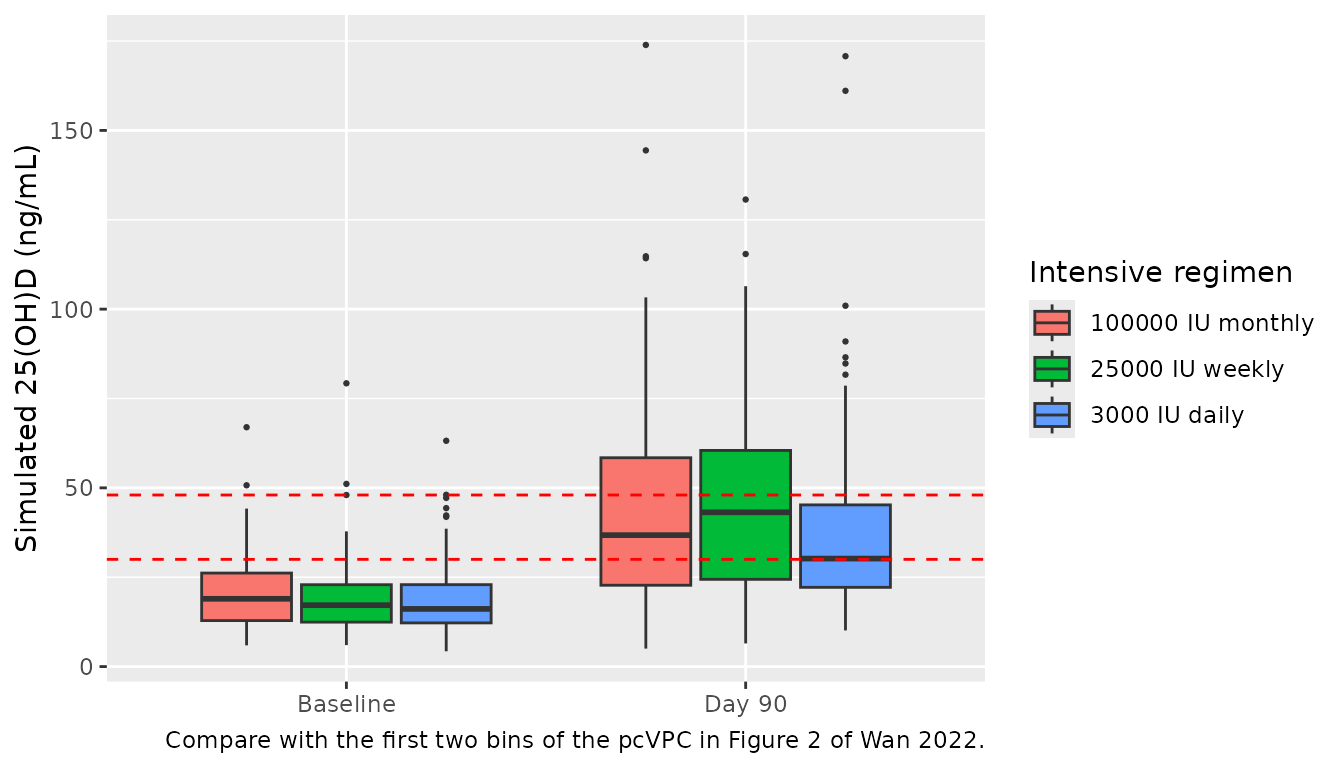
The simulated baseline (median about 17 ng/mL, 5th-95th percentile about 7-40 ng/mL) and the day-90 rise to a median in the mid-30s agree with the first two bins of the Figure 2 pcVPC.

PKNCA validation

Wan 2022 reports no NCA parameters. PKNCA is used here to summarise the three C3 intensive regimens for a typical 24 kg child, followed through a nine-month washout with no maintenance dose. The terminal half-life must equal log(2) * V/CL for this linear model: 283 days, because the basal amount and the dosed drug decay at the same rate once absorption is over.

ev_nca <- bind_rows(lapply(seq_len(nrow(arms)), function(k) {
  a <- arms[k, ]
  dose <- tibble(
    id = k, time = (seq_len(a$n_dose) - 1) * a$ii_day * 24,
    amt = a$amt_iu * ug_per_iu, evid = 1L, cmt = "depot"
  )
  obs <- tibble(id = k, time = seq(0, 365 * 24, by = 24), amt = 0, evid = 0L, cmt = "central")
  bind_rows(dose, obs) |> mutate(WT = 24, treatment = a$arm)
})) |>
  arrange(id, time, desc(evid))
sim_nca <- rxode2::rxSolve(mod_typical, ev_nca,
  keep = "treatment", rtol = 1e-10, atol = 1e-12, maxsteps = 1e6,
  returnType = "data.frame"
) |>
  dplyr::filter(!is.na(Cc)) |>
  select(id, time, Cc, treatment)
#> ℹ omega/sigma items treated as zero: 'etalcl', 'etalrbase'
#> Warning: multi-subject simulation without without 'omega'

conc_obj <- PKNCA::PKNCAconc(sim_nca, Cc ~ time | treatment + id)
dose_obj <- PKNCA::PKNCAdose(
  ev_nca |> filter(evid == 1) |> select(id, time, amt, treatment),
  amt ~ time | treatment + id
)
intervals <- data.frame(
  start = c(0, 120 * 24),
  end = c(90 * 24, 365 * 24),
  cmax = c(TRUE, FALSE),
  tmax = c(TRUE, FALSE),
  auclast = c(TRUE, FALSE),
  half.life = c(FALSE, TRUE)
)
nca_res <- PKNCA::pk.nca(PKNCA::PKNCAdata(conc_obj, dose_obj, intervals = intervals))
nca_df <- as.data.frame(nca_res)
nca_course <- nca_df |>
  filter(start == 0, PPTESTCD %in% c("cmax", "tmax", "auclast")) |>
  select(treatment, PPTESTCD, PPORRES) |>
  tidyr::pivot_wider(names_from = PPTESTCD, values_from = PPORRES)
nca_washout <- nca_df |>
  filter(start == 120 * 24, PPTESTCD == "half.life") |>
  select(treatment, half.life = PPORRES)
nca_tab <- inner_join(nca_course, nca_washout, by = "treatment") |>
  mutate(tmax_day = tmax / 24, half_life_day = half.life / 24)
nca_tab |>
  select(treatment, cmax, tmax_day, auclast, half_life_day) |>
  dplyr::rename(
    "Regimen" = treatment, "Cmax 0-90 d (ng/mL)" = cmax,
    "Tmax (days)" = tmax_day, "AUC0-90 d (ng*h/mL)" = auclast,
    "Terminal t1/2 (days)" = half_life_day
  ) |>
  knitr::kable(digits = 1, caption = "PKNCA summary, typical 24 kg child, intensive course then washout.")

PKNCA summary, typical 24 kg child, intensive course then washout.
Regimen	Cmax 0-90 d (ng/mL)	Tmax (days)	AUC0-90 d (ng*h/mL)	Terminal t1/2 (days)
100000 IU monthly	36.5	61	63920.9	283.5
25000 IU weekly	36.7	85	60029.9	283.5
3000 IU daily	32.6	90	54396.2	283.5


t_half_expected <- log(2) * 322 / 0.0328 / 24
# Mono-exponential washout, so PKNCA's log-linear fit recovers it to
# integration and fitting error (measured < 0.1%).
stopifnot(all(abs(nca_tab$half_life_day / t_half_expected - 1) < 0.02))

The three regimens deliver similar total doses over 90 days (6750, 8125 and 7500 ug for daily, weekly and monthly). The weekly and monthly regimens reach about the same Cmax (about 37 ng/mL). Daily dosing reaches about 33 ng/mL, at the end of the course. The monthly regimen has the largest AUC over the course, because each 2500 ug bolus arrives early in its interval. The terminal half-life is the same for all three regimens, as expected.

Assumptions and deviations

Final values from the supplementary control stream. The supplement gives the NONMEM model “with values set to final estimates”. Its CL/F (0.0328 L/h) is used instead of the rounded 0.033 L/h in Table 2. The Discussion quotes 0.0328 L/h as well.
Table 2 CV% is sqrt(omega). The Table 2 BSV and residual “%CV” values equal the square roots of the supplement’s $OMEGA and $SIGMA variances (sqrt(0.878) = 0.937, sqrt(0.117) = 0.342, sqrt(0.145) = 0.381). The variances are used directly. The CL-C0 covariance (-0.273, a correlation of -0.85) is printed only in the supplement.
No endogenous input. C0 is encoded exactly as the control stream has it, as an initial amount BC*V with no endogenous production term. In the model, an untreated child’s 25(OH)D therefore falls with the 283-day half-life, even though the paper describes C0 as reflecting endogenous production. The library keeps the published structure. Users simulating long untreated periods should be aware of this.
Dose units. The dose record is colecalciferol in ug (1 IU = 0.025 ug), per the supplement’s $INPUT. The model has no colecalciferol-to-25(OH)D molar conversion, matching the source.
Figure 3 and Figure 4 reference values were digitised by the maintainers from the publisher’s figure images. Each panel’s y-axis was calibrated on the 30 and 48 ng/mL target lines. Readings are good to about 1 ng/mL. Figure 3’s curves are smoothed, so peaks are compared loosely.
Figure 4 weight distribution. The CKiD-based virtual population used by the authors is not published. A uniform weight grid is used within each band, and the comparison is a bracket test rather than a point comparison.
Trial simulation. Only the first 3-month intensive course is simulated. The trial’s response-guided switch to maintenance or a repeated course is not reproduced. Weights are log-normal around the Table 1 median and IQR, truncated to 9-80 kg.
Covariates not retained. Scaled serum creatinine (CREAT relative to CREAT_REF) and glomerular disease (DIS_GLOMERULAR, documentation name only) are listed in covariatesDataExcluded. Neither has a published coefficient.
Errata. No correction notice for Wan 2022 was found on Europe PMC as of 2026-10-02.