Axomadol (Mangas-Sanjuan 2016)
Source:vignettes/articles/MangasSanjuan_2016_axomadol.Rmd
MangasSanjuan_2016_axomadol.RmdModel and source
- Citation: Mangas-Sanjuan V, Pastor JM, Rengelshausen J, Bursi R, Troconiz IF. (2016). Population pharmacokinetic/pharmacodynamic modelling of the effects of axomadol and its O-demethyl metabolite on pupil diameter and nociception in healthy subjects. Br J Clin Pharmacol 82(1):112-128. doi:10.1111/bcp.12921.
- Description: Semi-physiological population pharmacokinetic and joint pharmacodynamic model of axomadol (a racemic analgesic with opioid agonistic and monoamine-reuptake-inhibitor activity) and its O-demethyl (ODM) metabolite in healthy adult volunteers. The PK structure carries two parallel enantiomer chains (RR-suffix r and SS-suffix s), each consisting of a first-order absorption depot, a liver compartment mimicking first-pass conversion, a parent central compartment, and a metabolite central compartment. Within each enantiomer the parent and metabolite share a single apparent volume of distribution (VP = VM) and share a single typical first-order elimination rate constant (kP0 = kM0), although between-subject variability is estimated separately for the two elimination pathways. The PD layer is shared across the enantiomer chains and is driven by the SS parent in plasma (mydriatic Emax) and by the RR metabolite at a hysteresis effect site (linearly miotic). Pupil diameter is the sum of those two opposing effects; cold-pressor analgesic AUC is a linear function of the parent and metabolite contributions to pupil diameter. Parameter values are from Mangas-Sanjuan et al. 2016 Tables 2, 4, and 5.
- Article: Br J Clin Pharmacol 82(1):112-128 (2016)
Mangas-Sanjuan et al. characterised the pharmacokinetics and the pharmacodynamic effects of the racemic analgesic axomadol and its O-demethyl metabolite in healthy adult volunteers, linking pupil diameter (a PD biomarker reflecting opioid agonism and noradrenergic reuptake inhibition) to the cold-pressor analgesic AUC. The packaged model carries both enantiomer chains (RR + SS), each with a parent plasma compartment, a metabolite plasma compartment, and a liver compartment mimicking the first-pass conversion, plus a shared hysteresis effect site for the active RR metabolite and the joint PD layers for pupil diameter and cold-pressor AUC.
Population
The model was fit to pooled data from two Phase I trials in Caucasian
healthy volunteers (n = 74 per the Methods total; Table 1
dose-group counts sum to 72). Study A was a two-period crossover at 66
mg and 111 mg axomadol b.i.d. in 24 subjects (12 male, 14 female; age
46-64 y; mean weight 74.9 kg). Study B was a dose-escalation
parallel-group design at 100, 125, 150, and 150-then-225 mg axomadol
q12h-to-q8h in 48 subjects (24 male, 24 female; age 40-65 y; mean weight
71.1 kg). All subjects were CYP2D6 extensive metabolisers (subjects on
CYP2D6 inhibitors within the previous 4 weeks were excluded; Study A
used dextromethorphan urinary metabolic ratio for phenotyping and Study
B used TaqMan CYP2D6 allele genotyping).
The population metadata is available programmatically:
readModelDb("MangasSanjuan_2016_axomadol")$population.
Source trace
The per-parameter origin is recorded as an in-file comment next to
each ini() entry in
inst/modeldb/specificDrugs/MangasSanjuan_2016_axomadol.R.
The following table summarises the principal sources.
| Equation / parameter | Value | Source |
|---|---|---|
kgl_r, kgl_s (absorption rate, 1/h) |
1.68, 2.81 | Mangas-Sanjuan 2016 Table 2 |
klp_r, klp_s (liver-to-parent rate,
1/h) |
18.8, 18.0 | Mangas-Sanjuan 2016 Table 2 |
kpl_r, kpl_s (parent-to-liver rate,
1/h) |
0.0469, 0.0997 | Mangas-Sanjuan 2016 Table 2 |
kp0_r, kp0_s (parent + metabolite
elimination, 1/h) |
0.0793, 0.0894 | Mangas-Sanjuan 2016 Table 2 (kP0 = kM0 typical per footnote *) |
klm_r, klm_s (metabolite formation,
1/h) |
0.0115, 0.0157 | Mangas-Sanjuan 2016 Table 2 |
vc_r, vc_s (VP/F = VM/F, L) |
424, 528 | Mangas-Sanjuan 2016 Table 2; F fixed at 1 (Methods) |
tlag_r, tlag_s (lag time, h) |
0.26, 0.27 | Mangas-Sanjuan 2016 Table 2 |
| IIV (RR, SS) | 16-257% CV | Mangas-Sanjuan 2016 Table 2 |
pd0 (baseline pupil, mm) |
5.45 | Mangas-Sanjuan 2016 Table 4 |
emax, ec50 (SS-parent on pupil) |
0.79 mm, 90.7 ng/mL | Mangas-Sanjuan 2016 Table 4 |
ke0 (RR-metab effect-site, 1/h) |
0.0124 | Mangas-Sanjuan 2016 Table 4 (t1/2,ke0 ~ 55.9 h) |
slp2 (RR-metab effect-site slope, mm/(ng/mL)) |
9.67e-3 | Mangas-Sanjuan 2016 Table 4 |
| Pupil residual SD (mm) | 0.46 | Mangas-Sanjuan 2016 Table 4 |
aucbase (baseline cold-pressor AUC, pain unit*s) |
3760 | Mangas-Sanjuan 2016 Table 5 |
slp3 (RR-metab effect on AUC) |
0.0939 | Mangas-Sanjuan 2016 Table 5 |
slp4 (SS-parent effect on AUC) |
0.23 | Mangas-Sanjuan 2016 Table 5 |
| AUC residual SD (log(pain unit*s)) | 0.42 | Mangas-Sanjuan 2016 Table 5 |
| Pupil equation [1] | n/a | Mangas-Sanjuan 2016 page text after Table 3 |
| Cold-pressor equation [3] | n/a | Mangas-Sanjuan 2016 page text after Table 4 |
| Effect-compartment hysteresis equation | n/a | Sheiner 1979 (reference 24 in source) |
The plasma residual SDs encoded in the model file are the Study A
values: 0.20 (RR-parent), 0.26 (SS-parent), 0.17 (RR-metab), 0.14
(SS-metab) in log(ng/mL). Mangas-Sanjuan 2016 Table 2 also
reports Study B residual SDs (0.33, 0.49, 0.24, 0.27) which are larger
and not encoded here (the model carries a single residual per analyte
per Bender 2009 / Valitalo 2017 convention; the Study A column was
chosen as the more precise per-subject estimate).
Virtual cohort
The figures below use a deterministic typical-value simulation
(zeroRe()) to replicate the population-mean profiles of
Figure 5 and a small stochastic VPC to show the band of inter-subject
variability. The Mangas-Sanjuan 2016 analysis included no clinically
retained covariate effects so the cohort can be a single homogeneous
group; the differences between published-figure curves arise from the
enantiomer-specific PK and the joint PD structure.
set.seed(2026)

# Dose-event helper. The racemic axomadol dose is split 50/50 across
# the two enantiomer absorption depots, mirroring the Valitalo 2017
# ketorolac convention (no in vivo interconversion between
# enantiomers is modelled). The dose schedule below replicates the
# 225 mg b.i.d. arm of Study B over 3 weeks of treatment (Figure 5
# of the source paper).
build_axomadol_events <- function(n_subjects, dose_mg, tau_h,
                                  n_days, id_offset = 0L,
                                  obs_step_h = 1) {
  ids <- id_offset + seq_len(n_subjects)
  dose_times <- seq(0, by = tau_h, length.out = ceiling(n_days * 24 / tau_h))
  dose_per_enantiomer <- dose_mg / 2

  dose_r <- expand.grid(id = ids, time = dose_times,
                        stringsAsFactors = FALSE)
  dose_r$evid <- 1L
  dose_r$amt  <- dose_per_enantiomer
  dose_r$cmt  <- "depot_r"

  dose_s <- dose_r
  dose_s$cmt <- "depot_s"

  # Coarse 1 h observation grid keeps the 3-week simulation tractable
  # while still capturing peak / trough dynamics.
  obs_times <- seq(0, n_days * 24, by = obs_step_h)
  obs <- expand.grid(id = ids, time = obs_times,
                     stringsAsFactors = FALSE)
  obs$evid <- 0L
  obs$amt  <- 0
  obs$cmt  <- "Cc_s"  # any algebraic-observable name works; rxSolve
                      # returns every output (Cc_r, Cc_s, Cm_r,
                      # Cm_s, pdiameter, coldPressorAUC) as a column.

  out <- rbind(dose_r, dose_s, obs)
  out[order(out$id, out$time, -out$evid), ]
}

# Single multiple-dose cohort: 20 subjects on 225 mg b.i.d. for 21 days
# (Figure 5 reference regimen).
events_ss <- build_axomadol_events(n_subjects = 20L,
                                   dose_mg    = 225,
                                   tau_h      = 12,
                                   n_days     = 21,
                                   id_offset  = 0L)

# Sanity check: disjoint (id, time, evid) triples -- no duplicate dose
# or observation rows that would distort the simulation.
stopifnot(!anyDuplicated(unique(events_ss[, c("id", "time", "evid")])))
Simulation
mod <- readModelDb("MangasSanjuan_2016_axomadol")

# Typical-value simulation reproduces Mangas-Sanjuan 2016 Figure 5
# (no random effects, no residual error).
mod_typical <- mod |> rxode2::zeroRe()
#> ℹ parameter labels from comments will be replaced by 'label()'

sim_typical <- rxode2::rxSolve(mod_typical,
                               events    = events_ss
                               ) |>
  as.data.frame()
#> ℹ omega/sigma items treated as zero: 'etalkgl_r', 'etalkgl_s', 'etalkp0_r', 'etalkp0_s', 'etalkm0_r', 'etalkm0_s', 'etalklm_r', 'etalklm_s', 'etalvc_r', 'etalvc_s', 'etaltlag_r', 'etaltlag_s', 'etalpd0', 'etalslp2', 'etalec50', 'etalaucbase', 'etaltotal'
#> Warning: multi-subject simulation without without 'omega'

# Stochastic simulation overlays inter-subject variability.
sim_stoch <- rxode2::rxSolve(mod,
                             events    = events_ss
                             ) |>
  as.data.frame()
#> ℹ parameter labels from comments will be replaced by 'label()'
Replicate Mangas-Sanjuan 2016 Figure 5
Figure 5A – Plasma SS-parent and RR-metabolite + RR-metabolite effect-site
Replicates Figure 5A of Mangas-Sanjuan 2016, which shows that the SS parent reaches steady state in plasma within ~5 dosing intervals while the RR metabolite at the effect site approaches steady state much later (the equilibration half-life t1/2,ke0 ~ 55.9 h dominates).
fig5a <- sim_typical |>
  dplyr::filter(id == 1) |>
  dplyr::select(time, `SS parent (plasma)` = Cc_s,
                `RR metabolite (plasma)` = Cm_r,
                `RR metabolite (effect site)` = Cem_r) |>
  tidyr::pivot_longer(-time, names_to = "species", values_to = "conc")

ggplot(fig5a, aes(time / 24, conc, colour = species)) +
  geom_line(linewidth = 0.75) +
  labs(x = "Time (days)",
       y = "Concentration (ng/mL)",
       colour = NULL,
       caption = "Replicates Figure 5A of Mangas-Sanjuan 2016 (225 mg b.i.d. axomadol).") +
  theme_minimal() +
  theme(legend.position = "top")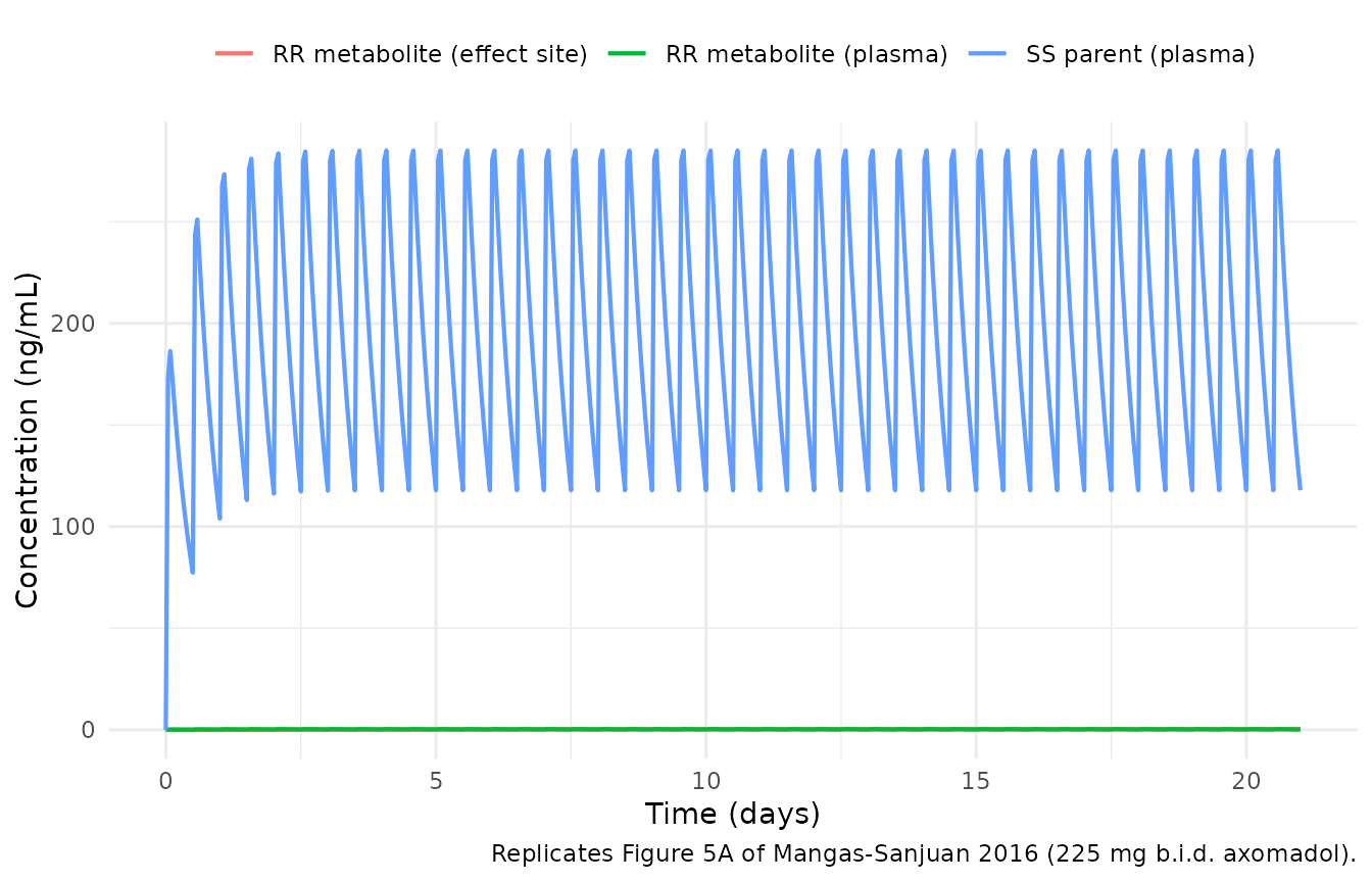
Figure 5B – Pupil diameter, SS-parent and RR-metabolite contributions
Replicates Figure 5B: the SS parent in plasma drives a rapid (within the first dosing interval) increase in pupil diameter via Emax, and the RR metabolite at the effect site drives a slow (over ~10 days) linear decrease. The net pupil diameter starts rising, then declines below baseline as the metabolite effect dominates at steady state.
fig5b <- sim_typical |>
  dplyr::filter(id == 1) |>
  dplyr::mutate(
    `Baseline`                      = pd0,
    `Net pupil diameter`            = pdiameter,
    `SS-parent contribution (+)`    = pd0 + e_parent_s,
    `RR-metabolite contribution (-)` = pd0 - e_metab_r
  ) |>
  dplyr::select(time, `Baseline`, `SS-parent contribution (+)`,
                `RR-metabolite contribution (-)`, `Net pupil diameter`) |>
  tidyr::pivot_longer(-time, names_to = "component",
                      values_to = "pupil_mm")

ggplot(fig5b, aes(time / 24, pupil_mm, colour = component)) +
  geom_line(linewidth = 0.75) +
  labs(x = "Time (days)",
       y = "Pupil diameter (mm)",
       colour = NULL,
       caption = "Replicates Figure 5B of Mangas-Sanjuan 2016 (225 mg b.i.d. axomadol).") +
  theme_minimal() +
  theme(legend.position = "top")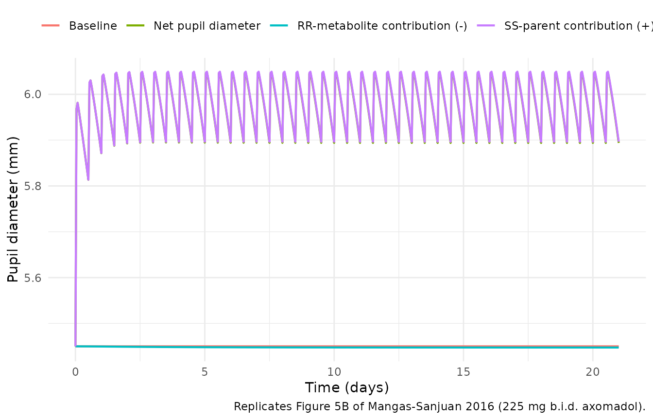
Figure 5C – Cold-pressor AUC, parent and metabolite contributions
Replicates Figure 5C: at steady state the SS parent and RR metabolite contribute roughly equally (~10-12% reduction each) to the cold-pressor analgesic AUC reduction, for a maximum overall reduction of ~20% after 3 weeks of dosing.
fig5c <- sim_typical |>
  dplyr::filter(id == 1) |>
  dplyr::mutate(
    rel_AUC_total  = coldPressorAUC                       / aucbase * 100,
    rel_AUC_parent = (aucbase - slp4 * e_parent_s)        / aucbase * 100,
    rel_AUC_metab  = (aucbase - slp3 * e_metab_r)         / aucbase * 100
  ) |>
  dplyr::select(time,
                `Net cold-pressor AUC (% of baseline)` = rel_AUC_total,
                `SS-parent contribution (% of baseline)`  = rel_AUC_parent,
                `RR-metabolite contribution (% of baseline)` = rel_AUC_metab) |>
  tidyr::pivot_longer(-time, names_to = "component",
                      values_to = "rel_AUC")

ggplot(fig5c, aes(time / 24, rel_AUC, colour = component)) +
  geom_line(linewidth = 0.75) +
  geom_hline(yintercept = 100, linetype = "dashed", colour = "grey50") +
  labs(x = "Time (days)",
       y = "Cold-pressor AUC (% of baseline)",
       colour = NULL,
       caption = "Replicates Figure 5C of Mangas-Sanjuan 2016 (225 mg b.i.d. axomadol).") +
  theme_minimal() +
  theme(legend.position = "top")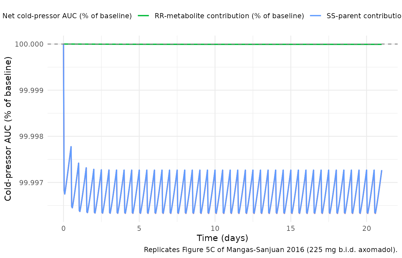
Visual predictive check (stochastic)
The single-subject typical-value figures above show the central tendency; the per-subject VPC below overlays the dispersion driven by the published between-subject variability on PK and PD parameters. The pupil-diameter band widens substantially after the first week as the high IIV on EC50 (CV = 257%) compounds with the metabolite slope IIV (CV = 84%).
sim_stoch |>
  dplyr::group_by(time) |>
  dplyr::summarise(
    q05 = quantile(pdiameter, 0.05, na.rm = TRUE),
    q50 = quantile(pdiameter, 0.50, na.rm = TRUE),
    q95 = quantile(pdiameter, 0.95, na.rm = TRUE),
    .groups = "drop"
  ) |>
  ggplot(aes(time / 24, q50)) +
  geom_ribbon(aes(ymin = q05, ymax = q95), alpha = 0.25,
              fill = "steelblue") +
  geom_line(linewidth = 0.75, colour = "steelblue4") +
  geom_hline(yintercept = 5.45, linetype = "dashed", colour = "grey50") +
  labs(x = "Time (days)",
       y = "Pupil diameter (mm)",
       caption = paste("VPC band: 5-95% across", length(unique(sim_stoch$id)),
                       "subjects with published IIV; dashed line = baseline 5.45 mm.")) +
  theme_minimal()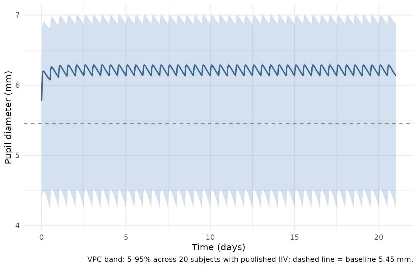
PKNCA validation – SS-parent steady-state
The cold-pressor and pupil-diameter PD relationships in Mangas-Sanjuan 2016 are driven by the SS-axomadol parent (the mydriatic component) and the RR O-demethyl-axomadol metabolite at its effect site (the miotic component). The SS parent is the active species for which an NCA-style summary is informative.
# PKNCA input: SS-parent plasma concentration, renamed to Cc as
# required by PKNCA + nlmixr2lib convention.
sim_nca <- sim_typical |>
  dplyr::filter(!is.na(Cc_s)) |>
  dplyr::transmute(id, time, Cc = Cc_s) |>
  dplyr::mutate(treatment = "225 mg axomadol b.i.d.")

# Guarantee a time = 0 row per (id, treatment) -- PKNCA needs an
# anchored AUC start.
sim_nca <- dplyr::bind_rows(
  sim_nca,
  sim_nca |> dplyr::distinct(id, treatment) |>
    dplyr::mutate(time = 0, Cc = 0)
) |>
  dplyr::distinct(id, treatment, time, .keep_all = TRUE) |>
  dplyr::arrange(id, treatment, time)

dose_df <- events_ss |>
  dplyr::filter(evid == 1, cmt == "depot_s") |>
  dplyr::transmute(id, time,
                   amt       = amt,
                   treatment = "225 mg axomadol b.i.d.")

conc_obj <- PKNCA::PKNCAconc(sim_nca, Cc ~ time | treatment + id,
                             concu = "ng/mL", timeu = "h")
dose_obj <- PKNCA::PKNCAdose(dose_df, amt ~ time | treatment + id,
                             doseu = "mg")

tau_h <- 12
ss_start <- max(dose_df$time)
intervals <- data.frame(
  start    = ss_start,
  end      = ss_start + tau_h,
  cmax     = TRUE,
  tmax     = TRUE,
  cmin     = TRUE,
  cav      = TRUE,
  auclast  = TRUE
)

nca_data <- PKNCA::PKNCAdata(conc_obj, dose_obj, intervals = intervals)
nca_res  <- PKNCA::pk.nca(nca_data)

knitr::kable(
  as.data.frame(nca_res),
  caption = paste("Steady-state NCA on SS-axomadol parent plasma",
                  "concentrations across the final 12 h dosing",
                  "interval (225 mg b.i.d., day 21 of 3 weeks).")
)| treatment | id | start | end | PPTESTCD | PPORRES | exclude | PPORRESU |
|---|---|---|---|---|---|---|---|
| 225 mg axomadol b.i.d. | 1 | 492 | 504 | auclast | 2381.4122 | NA | h*ng/mL |
| 225 mg axomadol b.i.d. | 1 | 492 | 504 | cmax | 285.0098 | NA | ng/mL |
| 225 mg axomadol b.i.d. | 1 | 492 | 504 | cmin | 117.8724 | NA | ng/mL |
| 225 mg axomadol b.i.d. | 1 | 492 | 504 | tmax | 2.0000 | NA | h |
| 225 mg axomadol b.i.d. | 1 | 492 | 504 | cav | 198.4510 | NA | ng/mL |
| 225 mg axomadol b.i.d. | 2 | 492 | 504 | auclast | 2381.4122 | NA | h*ng/mL |
| 225 mg axomadol b.i.d. | 2 | 492 | 504 | cmax | 285.0098 | NA | ng/mL |
| 225 mg axomadol b.i.d. | 2 | 492 | 504 | cmin | 117.8724 | NA | ng/mL |
| 225 mg axomadol b.i.d. | 2 | 492 | 504 | tmax | 2.0000 | NA | h |
| 225 mg axomadol b.i.d. | 2 | 492 | 504 | cav | 198.4510 | NA | ng/mL |
| 225 mg axomadol b.i.d. | 3 | 492 | 504 | auclast | 2381.4122 | NA | h*ng/mL |
| 225 mg axomadol b.i.d. | 3 | 492 | 504 | cmax | 285.0098 | NA | ng/mL |
| 225 mg axomadol b.i.d. | 3 | 492 | 504 | cmin | 117.8724 | NA | ng/mL |
| 225 mg axomadol b.i.d. | 3 | 492 | 504 | tmax | 2.0000 | NA | h |
| 225 mg axomadol b.i.d. | 3 | 492 | 504 | cav | 198.4510 | NA | ng/mL |
| 225 mg axomadol b.i.d. | 4 | 492 | 504 | auclast | 2381.4122 | NA | h*ng/mL |
| 225 mg axomadol b.i.d. | 4 | 492 | 504 | cmax | 285.0098 | NA | ng/mL |
| 225 mg axomadol b.i.d. | 4 | 492 | 504 | cmin | 117.8724 | NA | ng/mL |
| 225 mg axomadol b.i.d. | 4 | 492 | 504 | tmax | 2.0000 | NA | h |
| 225 mg axomadol b.i.d. | 4 | 492 | 504 | cav | 198.4510 | NA | ng/mL |
| 225 mg axomadol b.i.d. | 5 | 492 | 504 | auclast | 2381.4122 | NA | h*ng/mL |
| 225 mg axomadol b.i.d. | 5 | 492 | 504 | cmax | 285.0098 | NA | ng/mL |
| 225 mg axomadol b.i.d. | 5 | 492 | 504 | cmin | 117.8724 | NA | ng/mL |
| 225 mg axomadol b.i.d. | 5 | 492 | 504 | tmax | 2.0000 | NA | h |
| 225 mg axomadol b.i.d. | 5 | 492 | 504 | cav | 198.4510 | NA | ng/mL |
| 225 mg axomadol b.i.d. | 6 | 492 | 504 | auclast | 2381.4122 | NA | h*ng/mL |
| 225 mg axomadol b.i.d. | 6 | 492 | 504 | cmax | 285.0098 | NA | ng/mL |
| 225 mg axomadol b.i.d. | 6 | 492 | 504 | cmin | 117.8724 | NA | ng/mL |
| 225 mg axomadol b.i.d. | 6 | 492 | 504 | tmax | 2.0000 | NA | h |
| 225 mg axomadol b.i.d. | 6 | 492 | 504 | cav | 198.4510 | NA | ng/mL |
| 225 mg axomadol b.i.d. | 7 | 492 | 504 | auclast | 2381.4122 | NA | h*ng/mL |
| 225 mg axomadol b.i.d. | 7 | 492 | 504 | cmax | 285.0098 | NA | ng/mL |
| 225 mg axomadol b.i.d. | 7 | 492 | 504 | cmin | 117.8724 | NA | ng/mL |
| 225 mg axomadol b.i.d. | 7 | 492 | 504 | tmax | 2.0000 | NA | h |
| 225 mg axomadol b.i.d. | 7 | 492 | 504 | cav | 198.4510 | NA | ng/mL |
| 225 mg axomadol b.i.d. | 8 | 492 | 504 | auclast | 2381.4122 | NA | h*ng/mL |
| 225 mg axomadol b.i.d. | 8 | 492 | 504 | cmax | 285.0098 | NA | ng/mL |
| 225 mg axomadol b.i.d. | 8 | 492 | 504 | cmin | 117.8724 | NA | ng/mL |
| 225 mg axomadol b.i.d. | 8 | 492 | 504 | tmax | 2.0000 | NA | h |
| 225 mg axomadol b.i.d. | 8 | 492 | 504 | cav | 198.4510 | NA | ng/mL |
| 225 mg axomadol b.i.d. | 9 | 492 | 504 | auclast | 2381.4122 | NA | h*ng/mL |
| 225 mg axomadol b.i.d. | 9 | 492 | 504 | cmax | 285.0098 | NA | ng/mL |
| 225 mg axomadol b.i.d. | 9 | 492 | 504 | cmin | 117.8724 | NA | ng/mL |
| 225 mg axomadol b.i.d. | 9 | 492 | 504 | tmax | 2.0000 | NA | h |
| 225 mg axomadol b.i.d. | 9 | 492 | 504 | cav | 198.4510 | NA | ng/mL |
| 225 mg axomadol b.i.d. | 10 | 492 | 504 | auclast | 2381.4122 | NA | h*ng/mL |
| 225 mg axomadol b.i.d. | 10 | 492 | 504 | cmax | 285.0098 | NA | ng/mL |
| 225 mg axomadol b.i.d. | 10 | 492 | 504 | cmin | 117.8724 | NA | ng/mL |
| 225 mg axomadol b.i.d. | 10 | 492 | 504 | tmax | 2.0000 | NA | h |
| 225 mg axomadol b.i.d. | 10 | 492 | 504 | cav | 198.4510 | NA | ng/mL |
| 225 mg axomadol b.i.d. | 11 | 492 | 504 | auclast | 2381.4122 | NA | h*ng/mL |
| 225 mg axomadol b.i.d. | 11 | 492 | 504 | cmax | 285.0098 | NA | ng/mL |
| 225 mg axomadol b.i.d. | 11 | 492 | 504 | cmin | 117.8724 | NA | ng/mL |
| 225 mg axomadol b.i.d. | 11 | 492 | 504 | tmax | 2.0000 | NA | h |
| 225 mg axomadol b.i.d. | 11 | 492 | 504 | cav | 198.4510 | NA | ng/mL |
| 225 mg axomadol b.i.d. | 12 | 492 | 504 | auclast | 2381.4122 | NA | h*ng/mL |
| 225 mg axomadol b.i.d. | 12 | 492 | 504 | cmax | 285.0098 | NA | ng/mL |
| 225 mg axomadol b.i.d. | 12 | 492 | 504 | cmin | 117.8724 | NA | ng/mL |
| 225 mg axomadol b.i.d. | 12 | 492 | 504 | tmax | 2.0000 | NA | h |
| 225 mg axomadol b.i.d. | 12 | 492 | 504 | cav | 198.4510 | NA | ng/mL |
| 225 mg axomadol b.i.d. | 13 | 492 | 504 | auclast | 2381.4122 | NA | h*ng/mL |
| 225 mg axomadol b.i.d. | 13 | 492 | 504 | cmax | 285.0098 | NA | ng/mL |
| 225 mg axomadol b.i.d. | 13 | 492 | 504 | cmin | 117.8724 | NA | ng/mL |
| 225 mg axomadol b.i.d. | 13 | 492 | 504 | tmax | 2.0000 | NA | h |
| 225 mg axomadol b.i.d. | 13 | 492 | 504 | cav | 198.4510 | NA | ng/mL |
| 225 mg axomadol b.i.d. | 14 | 492 | 504 | auclast | 2381.4122 | NA | h*ng/mL |
| 225 mg axomadol b.i.d. | 14 | 492 | 504 | cmax | 285.0098 | NA | ng/mL |
| 225 mg axomadol b.i.d. | 14 | 492 | 504 | cmin | 117.8724 | NA | ng/mL |
| 225 mg axomadol b.i.d. | 14 | 492 | 504 | tmax | 2.0000 | NA | h |
| 225 mg axomadol b.i.d. | 14 | 492 | 504 | cav | 198.4510 | NA | ng/mL |
| 225 mg axomadol b.i.d. | 15 | 492 | 504 | auclast | 2381.4122 | NA | h*ng/mL |
| 225 mg axomadol b.i.d. | 15 | 492 | 504 | cmax | 285.0098 | NA | ng/mL |
| 225 mg axomadol b.i.d. | 15 | 492 | 504 | cmin | 117.8724 | NA | ng/mL |
| 225 mg axomadol b.i.d. | 15 | 492 | 504 | tmax | 2.0000 | NA | h |
| 225 mg axomadol b.i.d. | 15 | 492 | 504 | cav | 198.4510 | NA | ng/mL |
| 225 mg axomadol b.i.d. | 16 | 492 | 504 | auclast | 2381.4122 | NA | h*ng/mL |
| 225 mg axomadol b.i.d. | 16 | 492 | 504 | cmax | 285.0098 | NA | ng/mL |
| 225 mg axomadol b.i.d. | 16 | 492 | 504 | cmin | 117.8724 | NA | ng/mL |
| 225 mg axomadol b.i.d. | 16 | 492 | 504 | tmax | 2.0000 | NA | h |
| 225 mg axomadol b.i.d. | 16 | 492 | 504 | cav | 198.4510 | NA | ng/mL |
| 225 mg axomadol b.i.d. | 17 | 492 | 504 | auclast | 2381.4122 | NA | h*ng/mL |
| 225 mg axomadol b.i.d. | 17 | 492 | 504 | cmax | 285.0098 | NA | ng/mL |
| 225 mg axomadol b.i.d. | 17 | 492 | 504 | cmin | 117.8724 | NA | ng/mL |
| 225 mg axomadol b.i.d. | 17 | 492 | 504 | tmax | 2.0000 | NA | h |
| 225 mg axomadol b.i.d. | 17 | 492 | 504 | cav | 198.4510 | NA | ng/mL |
| 225 mg axomadol b.i.d. | 18 | 492 | 504 | auclast | 2381.4122 | NA | h*ng/mL |
| 225 mg axomadol b.i.d. | 18 | 492 | 504 | cmax | 285.0098 | NA | ng/mL |
| 225 mg axomadol b.i.d. | 18 | 492 | 504 | cmin | 117.8724 | NA | ng/mL |
| 225 mg axomadol b.i.d. | 18 | 492 | 504 | tmax | 2.0000 | NA | h |
| 225 mg axomadol b.i.d. | 18 | 492 | 504 | cav | 198.4510 | NA | ng/mL |
| 225 mg axomadol b.i.d. | 19 | 492 | 504 | auclast | 2381.4122 | NA | h*ng/mL |
| 225 mg axomadol b.i.d. | 19 | 492 | 504 | cmax | 285.0098 | NA | ng/mL |
| 225 mg axomadol b.i.d. | 19 | 492 | 504 | cmin | 117.8724 | NA | ng/mL |
| 225 mg axomadol b.i.d. | 19 | 492 | 504 | tmax | 2.0000 | NA | h |
| 225 mg axomadol b.i.d. | 19 | 492 | 504 | cav | 198.4510 | NA | ng/mL |
| 225 mg axomadol b.i.d. | 20 | 492 | 504 | auclast | 2381.4122 | NA | h*ng/mL |
| 225 mg axomadol b.i.d. | 20 | 492 | 504 | cmax | 285.0098 | NA | ng/mL |
| 225 mg axomadol b.i.d. | 20 | 492 | 504 | cmin | 117.8724 | NA | ng/mL |
| 225 mg axomadol b.i.d. | 20 | 492 | 504 | tmax | 2.0000 | NA | h |
| 225 mg axomadol b.i.d. | 20 | 492 | 504 | cav | 198.4510 | NA | ng/mL |
Mangas-Sanjuan 2016 does not report a NCA table for SS axomadol; the simulated NCA above is provided as a self-consistency check rather than a comparison-against-published metric. The order of magnitude is consistent with the visual range of Figure 5A (SS-parent steady-state concentration ~100-200 ng/mL).
Assumptions and deviations
- Race / ethnicity. The source paper reports only Caucasian volunteers; race / ethnicity does not enter the model and the cohort above does not stratify by race.
- CYP2D6 phenotype. All subjects in the source studies were extensive CYP2D6 metabolisers (poor metabolisers excluded); metaboliser status does not enter the model and dose-level was shown by the source authors not to affect any PK or PD parameter, so the cohort is run as a single homogeneous group.
- Bioavailability F. F is fixed at 1 (Methods: “the typical unknown absolute bioavailability F was assumed to be complete”) and carries no inter-individual variability in the final model (Population PK modelling: “Interindividual variability was supported in all model parameters except […] Relative Bioavailability parameter (F1)”).
-
Volume constraint. The apparent parent and
metabolite volumes of distribution of the same enantiomer are
constrained equal (
VP = VM; Methods) to avoid non-identifiability. Within each enantiomer the parent and metabolite sharevc_r(RR) orvc_s(SS); across enantiomers the volumes differ (RR 424 L, SS 528 L). -
Elimination-rate constraint. The parent and
metabolite typical elimination rates within each enantiomer are
constrained equal (
kP0 = kM0; Table 2 footnote *: “different estimates […] did not improve the fit significantly”). However the IIV variances on the two pathways are separately estimated; the model file encodes them asetalkp0_*(on parent elimination) andetalkm0_*(on metabolite elimination), with both etas drawing on the same shared typical valuelkp0_*and the cross-eta typical-value sharing declared via thepaper_specific_etasmetadata field. -
Combined-effect IIV. Mangas-Sanjuan 2016 Table 5
reports a single 93%-CV IIV on the joint cold-pressor term
[SLP3 * E_RR-m + SLP4 * E_SS-p]rather than two separate IIVs. The model file encodes this asetaltotal, applied multiplicatively to bothslp3andslp4per the paper’s parameterisation. -
Plasma residual SDs. Each analyte (RR-parent,
SS-parent, RR-metabolite, SS-metabolite) was fit with study-specific
residual variance in the source paper (one value per study, two
studies). The model file encodes the Study A values; the Study B
residuals (0.33, 0.49, 0.24, 0.27 in
log(ng/mL)) are documented above. -
Effect-compartment parameterisation. The Sheiner
1979 effect- compartment model with implicit-volume parameterisation
(
d Ce / dt = ke0 * (Cm_r - Ce)) is used; the effect-site compartment carries the concentration of the active RR metabolite directly, soCem_r = effect_odm_r. -
Compartment naming. The metabolite plasma
compartments (
central_odm_r,central_odm_s) and the effect compartment (effect_odm_r) carry the paper’s_odm(O-demethyl-axomadol) designator. The token is not yet a registered metabolite suffix ininst/references/compartment-names.md; the model file declares these three states via thepaper_specific_compartmentsmetadata field so the compartment-name convention check accepts them. -
Coupled enantiomer chains in one model file.
Mangas-Sanjuan 2016 fitted the RR and SS enantiomers as two parallel PK
problems, then a single joint PD layer on top using individual predicted
concentrations. The model file replicates this as one combined
rxode2model so that simulation produces both enantiomers and both PD outputs from one call; users who want the separate per-enantiomer typical-value parameters can read them fromreadModelDb("MangasSanjuan_2016_axomadol")$ini.