Risankizumab (Suleiman 2018) • nlmixr2lib

library(nlmixr2lib)
library(rxode2)
#> rxode2 5.1.2 using 2 threads (see ?getRxThreads)
#>   no cache: create with `rxCreateCache()`
library(dplyr)
#> 
#> Attaching package: 'dplyr'
#> The following objects are masked from 'package:stats':
#> 
#>     filter, lag
#> The following objects are masked from 'package:base':
#> 
#>     intersect, setdiff, setequal, union
library(tidyr)
library(ggplot2)
library(PKNCA)
#> 
#> Attaching package: 'PKNCA'
#> The following object is masked from 'package:stats':
#> 
#>     filter

Risankizumab population PK in psoriasis and Crohn’s disease (phase I-II)

Simulate risankizumab concentration-time profiles using the final population PK model of Suleiman et al. (2018) from the pooled analysis of one phase I study in psoriasis (Study 1, n=31), one phase II study in psoriasis (Study 2, n=126), and one phase II study in Crohn’s disease (Study 3, n=115). The source paper pooled 2831 plasma concentrations from 272 individuals across the three studies.

The model is a two-compartment structure with first-order subcutaneous absorption and linear elimination (NONMEM ADVAN4). Typical parameters for a 70 kg reference subject with baseline albumin 40 g/L (the overall cohort median) are CL = 0.30 L/day, Vc = 5.66 L, Vp = 3.43 L, Q = 0.33 L/day, ka = 0.18 /day, and F = 0.72. The final covariate set is body weight on CL, Q, Vc, and Vp (two shared exponents: 0.93 for CL/Q and 0.99 for Vc/Vp) and baseline serum albumin on CL (exponent -1.54).

Citation: Suleiman AA, Khatri A, Minocha M, Othman AA. Population Pharmacokinetics of the Interleukin-23 Inhibitor Risankizumab in Subjects with Psoriasis and Crohn’s Disease: Analyses of Phase I and II Trials. Clin Pharmacokinet. 2018;57(10):1259-1270. doi:10.1007/s40262-018-0704-z
Article: https://doi.org/10.1007/s40262-018-0704-z

Source trace

Per-parameter origins are recorded as in-file comments in the model file; the table below collects them in one place.

Equation / parameter	Value	Source location
Two-compartment ODE structure (ka -> central <-> peripheral1, linear CL)	n/a	Sect. 2.3.2 and 3.2 (NONMEM ADVAN4)
CL (typical, 70 kg, 40 g/L ALB)	0.30 L/day	Table 3
Vc (typical, 70 kg)	5.66 L	Table 3
Q (typical, 70 kg)	0.33 L/day	Table 3
Vp (typical, 70 kg)	3.43 L	Table 3
ka (typical)	0.18 /day	Table 3
F (SC absolute bioavailability)	0.72	Table 3
WT on CL and Q (shared exponent)	(WT/70)^0.93	Table 3; Eq. 3
WT on Vc and Vp (shared exponent)	(WT/70)^0.99	Table 3
ALB on CL	(ALB/40)^-1.54	Table 3; Eq. 4; ALB reference = overall Table 2 median 40 g/L
IIV CL	37% CV -> omega^2 = log(1 + 0.37^2) = 0.12832	Table 3 (footnote b conversion)
IIV Vc	55% CV -> omega^2 = log(1 + 0.55^2) = 0.26432	Table 3
IIV Vp	35% CV -> omega^2 = log(1 + 0.35^2) = 0.11556	Table 3
IIV ka	80% CV -> omega^2 = log(1 + 0.80^2) = 0.49470	Table 3
IIV CL-Vc covariance	0.07182 (correlation 39%)	Sibling Suleiman 2019 Table 3 (non-paper provenance; see Assumptions)
Residual error	proportional, propSd = 0.19 (19% CV)	Sibling Suleiman 2019 Table 3 (non-paper provenance; see Assumptions)
Dosing regimen (psoriasis phase III)	150 mg SC weeks 0 and 4, then q12w	Sect. 2.3.4
Dosing regimen (Crohn’s phase II maintenance)	IV 600 mg weeks 0, 4, 8 induction, then SC 180 mg q8w	Sect. 2.3.4

Covariate column naming

Source column	Canonical column used here
`WT` (kg)	`WT` (kg; per `covariate-columns.md`)
`ALB` (g/L)	`ALB` (g/L; canonical general-scope)

Virtual population

Approximate the pooled Suleiman 2018 cohort (Table 2): median body weight 79 kg (range 36-138), overall albumin median 40 g/L (range 24-51). The paper simulates 100,000 virtual subjects per indication; the vignette uses 500 for a fast render.

set.seed(2018)
n_subj <- 500

pop <- tibble(
  ID  = seq_len(n_subj),
  WT  = pmin(pmax(rlnorm(n_subj, log(79), 0.26), 36), 138),  # kg
  ALB = pmin(pmax(rnorm(n_subj, 40, 4.5), 24), 51)           # g/L
)

Dosing dataset

Psoriasis phase III regimen (Sect. 2.3.4): 150 mg SC at weeks 0 and 4, then every 12 weeks (q12w) thereafter. Simulate through week 52.

dose_weeks <- c(0, 4, 16, 28, 40)
dose_times <- dose_weeks * 7

obs_times <- sort(unique(c(
  seq(0,  28,       by = 0.5),
  seq(28, 52 * 7,   by = 2)
)))

d_dose <- pop %>%
  crossing(TIME = dose_times) %>%
  mutate(AMT = 150, EVID = 1, CMT = 1, DV = NA_real_)

d_obs <- pop %>%
  crossing(TIME = obs_times) %>%
  mutate(AMT = NA_real_, EVID = 0, CMT = 2, DV = NA_real_)

d_sim <- bind_rows(d_dose, d_obs) %>%
  arrange(ID, TIME, desc(EVID)) %>%
  as.data.frame()

Simulate

mod <- readModelDb("Suleiman_2018_risankizumab")
sim <- rxSolve(mod, d_sim, returnType = "data.frame")
#> ℹ parameter labels from comments will be replaced by 'label()'

Concentration-time profile (replicates Fig. 2, Suleiman 2018)

sim_summary <- sim %>%
  filter(time > 0) %>%
  group_by(time) %>%
  summarise(
    median = median(Cc, na.rm = TRUE),
    lo     = quantile(Cc, 0.05, na.rm = TRUE),
    hi     = quantile(Cc, 0.95, na.rm = TRUE),
    .groups = "drop"
  )

ggplot(sim_summary, aes(x = time / 7)) +
  geom_ribbon(aes(ymin = lo, ymax = hi), alpha = 0.2, fill = "steelblue") +
  geom_line(aes(y = median), colour = "steelblue", linewidth = 1) +
  scale_y_log10() +
  labs(
    x        = "Time (weeks)",
    y        = "Risankizumab concentration (ug/mL)",
    title    = "Simulated risankizumab PK (150 mg SC weeks 0, 4, q12w)",
    subtitle = "Median and 90% prediction interval (N = 500 virtual pooled subjects)",
    caption  = "Replicates Fig. 2 of Suleiman 2018 (phase II psoriasis VPC layout)."
  ) +
  theme_bw()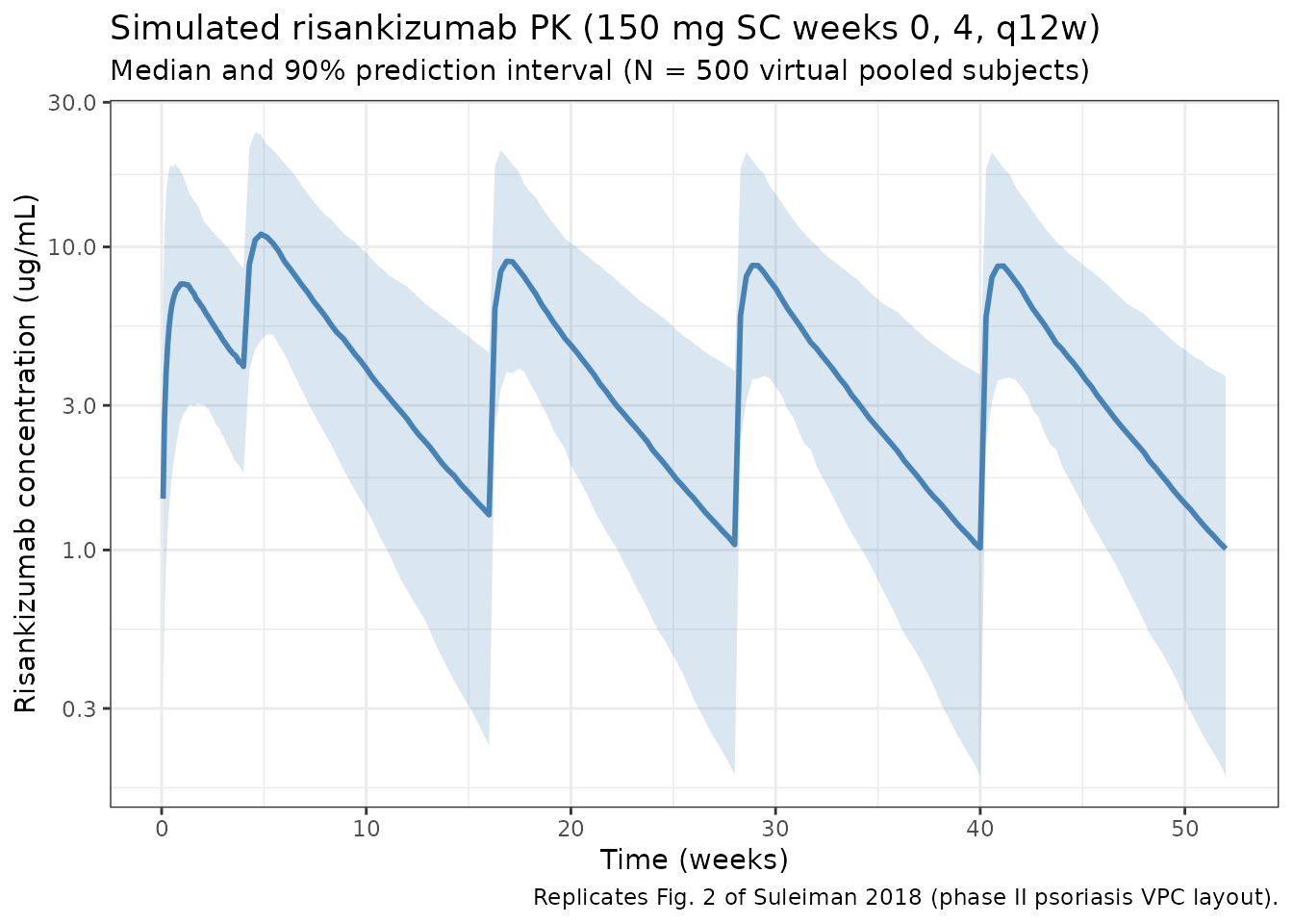

Typical-subject comparison against the published abstract

The Abstract gives typical values for two reference subjects (with random effects zeroed): (a) 90 kg psoriasis patient, ALB 42 g/L -> CL = 0.35 L/day, Vc = 7.26 L, Vp = 4.39 L, Vss = 11.7 L, terminal half-life ~27 days; (b) 65 kg Crohn’s patient, ALB 37 g/L -> CL = 0.31 L/day, Vc = 5.26 L, Vp = 3.19 L, Vss = 8.45 L, terminal half-life ~22 days. Reproduce these using the packaged model:

mod_typ <- rxode2::zeroRe(mod)
#> ℹ parameter labels from comments will be replaced by 'label()'

typ_scenarios <- tribble(
  ~scenario,           ~WT, ~ALB, ~paper_CL, ~paper_Vc, ~paper_Vp, ~paper_Vss, ~paper_thalf,
  "90 kg psoriasis",    90,   42,      0.35,      7.26,      4.39,       11.7,           27,
  "65 kg Crohn's",      65,   37,      0.31,      5.26,      3.19,       8.45,           22
)

# Closed-form typical values from the model equations.
lam_terminal <- function(kel, q, vc, vp) {
  k12 <- q / vc
  k21 <- q / vp
  s   <- kel + k12 + k21
  (s - sqrt(s^2 - 4 * kel * k21)) / 2
}

typ_calc <- typ_scenarios %>%
  rowwise() %>%
  mutate(
    calc_CL = 0.30 * (WT / 70)^0.93 * (ALB / 40)^(-1.54),
    calc_Vc = 5.66 * (WT / 70)^0.99,
    calc_Vp = 3.43 * (WT / 70)^0.99,
    calc_Q  = 0.33 * (WT / 70)^0.93,
    calc_Vss = calc_Vc + calc_Vp,
    calc_kel = calc_CL / calc_Vc,
    calc_thalf = log(2) / lam_terminal(calc_kel, calc_Q, calc_Vc, calc_Vp)
  ) %>%
  ungroup()

knitr::kable(
  typ_calc %>%
    transmute(
      scenario,
      `CL (paper / calc)`   = sprintf("%.2f / %.3f", paper_CL,   calc_CL),
      `Vc (paper / calc)`   = sprintf("%.2f / %.2f", paper_Vc,   calc_Vc),
      `Vp (paper / calc)`   = sprintf("%.2f / %.2f", paper_Vp,   calc_Vp),
      `Vss (paper / calc)`  = sprintf("%.2f / %.2f", paper_Vss,  calc_Vss),
      `t1/2 (paper / calc, days)` = sprintf("%.1f / %.1f", paper_thalf, calc_thalf)
    ),
  caption = "Suleiman 2018 typical-subject reference cases (Abstract vs closed-form derivation from the packaged model)."
)

Suleiman 2018 typical-subject reference cases (Abstract vs closed-form derivation from the packaged model).
scenario	CL (paper / calc)	Vc (paper / calc)	Vp (paper / calc)	Vss (paper / calc)	t1/2 (paper / calc, days)
90 kg psoriasis	0.35 / 0.352	7.26 / 7.26	4.39 / 4.40	11.70 / 11.66	27.0 / 26.3
65 kg Crohn’s	0.31 / 0.316	5.26 / 5.26	3.19 / 3.19	8.45 / 8.45	22.0 / 21.9

PKNCA validation

Run PKNCA on a steady-state 12-week maintenance interval of the psoriasis phase III regimen (weeks 16-28). The paper’s Abstract reports steady-state AUC(weeks 40-52) = 344 +/- 151 ug*day/mL for the psoriasis regimen; PKNCA on the 500-subject virtual cohort should be in a comparable range.

nca_conc <- sim %>%
  filter(time >= 16 * 7, time <= 28 * 7) %>%
  mutate(
    time_rel  = time - 16 * 7,
    treatment = "risankizumab_150mg_q12w"
  ) %>%
  rename(ID = id) %>%
  select(ID, time_rel, Cc, treatment)

nca_dose <- pop %>%
  mutate(
    time_rel  = 0,
    AMT       = 150,
    treatment = "risankizumab_150mg_q12w"
  ) %>%
  select(ID, time_rel, AMT, treatment)

conc_obj <- PKNCAconc(nca_conc, Cc ~ time_rel | treatment + ID)
dose_obj <- PKNCAdose(nca_dose, AMT ~ time_rel | treatment + ID)
data_obj <- PKNCAdata(
  conc_obj,
  dose_obj,
  intervals = data.frame(
    start     = 0,
    end       = 12 * 7,
    cmax      = TRUE,
    tmax      = TRUE,
    auclast   = TRUE,
    half.life = TRUE
  )
)
nca_results <- pk.nca(data_obj)
nca_summary <- summary(nca_results)
knitr::kable(
  nca_summary,
  digits  = 2,
  caption = "PKNCA summary for the steady-state maintenance interval (weeks 16-28) of the psoriasis phase III 150 mg SC q12w regimen."
)

PKNCA summary for the steady-state maintenance interval (weeks 16-28) of the psoriasis phase III 150 mg SC q12w regimen.
start	end	treatment	N	auclast	cmax	tmax	half.life
0	84	risankizumab_150mg_q12w	500	333 [50.8]	9.44 [50.7]	8.00 [2.00, 24.0]	28.6 [11.9]

Weight-effect sensitivity (replicates Fig. 4, Suleiman 2018)

Suleiman 2018 Fig. 4 shows the exposure ratio vs a reference subject across body weight and albumin strata. Reproduce the body-weight arm by simulating typical subjects at 60, 79 (cohort median), and 100 kg with ALB fixed at the cohort median.

wt_grid <- c(60, 79, 100)

wt_scenarios <- tibble(WT = wt_grid, ALB = 40)

wt_typ <- wt_scenarios %>%
  rowwise() %>%
  do({
    row <- .
    typ_pop <- tibble(ID = 1L, WT = row$WT, ALB = row$ALB)
    events <- bind_rows(
      typ_pop %>% crossing(TIME = dose_times) %>%
        mutate(AMT = 150, EVID = 1, CMT = 1, DV = NA_real_),
      typ_pop %>% crossing(TIME = obs_times) %>%
        mutate(AMT = NA_real_, EVID = 0, CMT = 2, DV = NA_real_)
    ) %>%
      arrange(TIME, desc(EVID)) %>%
      as.data.frame()
    df <- rxSolve(mod_typ, events, returnType = "data.frame") %>%
      filter(time >= 16 * 7, time <= 28 * 7, Cc > 0) %>%
      arrange(time)
    auctau <- sum(diff(df$time) * (head(df$Cc, -1) + tail(df$Cc, -1)) / 2)
    tibble(WT = row$WT, ALB = row$ALB, AUCtau = auctau)
  }) %>%
  bind_rows()
#> ℹ omega/sigma items treated as zero: 'etalcl', 'etalvc', 'etalvp', 'etalka'
#> ℹ omega/sigma items treated as zero: 'etalcl', 'etalvc', 'etalvp', 'etalka'
#> ℹ omega/sigma items treated as zero: 'etalcl', 'etalvc', 'etalvp', 'etalka'

ref_auc <- wt_typ$AUCtau[wt_typ$WT == 79]

wt_typ <- wt_typ %>%
  mutate(ratio = AUCtau / ref_auc)

knitr::kable(
  wt_typ,
  digits  = 2,
  caption = "Typical-subject AUCtau (weeks 16-28) vs body weight; ratios relative to the cohort-median 79 kg subject. Consistent with Fig. 4 of Suleiman 2018 which shows heavier subjects (>100 kg) exposed to ~25% lower AUC."
)

Typical-subject AUCtau (weeks 16-28) vs body weight; ratios relative to the cohort-median 79 kg subject. Consistent with Fig. 4 of Suleiman 2018 which shows heavier subjects (>100 kg) exposed to ~25% lower AUC.
WT	ALB	AUCtau	ratio
60	40	425.93	1.29
79	40	330.14	1.00
100	40	265.40	0.80

Assumptions and deviations

Reference albumin 40 g/L (non-paper-explicit). Suleiman 2018 Eq. 4 ((cov / median)^theta) is defined in terms of the covariate’s median, but Table 3 does not print the reference value used. The overall Table 2 median (40 g/L) was verified by back-calculating the paper’s typical-subject CL: 0.30 * (90/70)^0.93 * (42/40)^-1.54 = 0.351 L/day matches the Abstract’s 0.35 L/day for a typical 90 kg psoriasis subject with ALB 42 g/L, and 0.30 * (65/70)^0.93 * (37/40)^-1.54 = 0.314 L/day matches 0.31 L/day for a 65 kg Crohn’s subject with ALB 37 g/L.
Proportional residual error (propSd = 0.19) is non-paper provenance. Suleiman 2018 Sect. 3.2 states “Residual variability was best described by a proportional error model” but Table 3 does not report the magnitude; the value is expected to be in the paper’s Electronic Supplementary Material, which was not on disk during extraction. The packaged value 0.19 is carried from the sibling Suleiman_2019_risankizumab model in the same registry: same first author (Suleiman AA) and same authorship group (Khatri, Minocha, Othman), same drug, and the 2018 phase I-II cohort is a strict subset of the 2019 integrated phase I-III cohort used to fit the 2019 model. This substitution was authorised via sidecar requests 001/002 (option C).
CL-Vc covariance (0.07182, correlation 39%) is non-paper provenance. Suleiman 2018 Sect. 3.2 states “introducing a correlation between CL and Vc reduced the OFV by 135 points” but Table 3 reports only IIV variances, not the off-diagonal. The correlation is expected to be in the unavailable ESM. The packaged correlation (39%) is carried from Suleiman_2019_risankizumab Table 3 under the same sibling-substitution reasoning above; covariance = 0.39 * sqrt(0.12832 * 0.26432) = 0.07182 given the 2018 IIV variances.
Virtual population approximates the pooled Table 2 demographics. Suleiman 2018 does not publish individual-level data. Body weight is sampled log-normal around the pooled 79 kg median with SD 0.26 on the log scale (clipped to the observed 36-138 kg range). Albumin is sampled normally around the pooled 40 g/L median with SD 4.5 (clipped to the observed 24-51 g/L range). No correlation between WT and ALB is imposed; the paper does not report the joint distribution.
Disease population (psoriasis vs Crohn’s) is not a model covariate. The paper explicitly finds no residual pharmacokinetic difference between psoriasis and Crohn’s disease after accounting for body weight and albumin (Abstract, Conclusions), so the packaged model does not carry an indication indicator.
Sex, age, race, C-reactive protein, ALT, AST, serum creatinine, creatinine clearance, and ADA / NAb status were evaluated in the paper (Sect. 2.3.2) but were not retained in the final model and are not part of the packaged model.
Time-varying ADA covariate. Suleiman 2018 tested ADA status as binary, ADA titer as continuous, and time-varying LOCF-imputed binary; none were retained. The later Suleiman 2019 paper (Suleiman_2019_risankizumab) does carry an ADA titer threshold effect (>= 128 -> +43% CL) which was estimated from a much larger ADA-positive subgroup in phase III. Users wanting an ADA-sensitive risankizumab model should use the 2019 sibling.

Reference

Suleiman AA, Khatri A, Minocha M, Othman AA. Population Pharmacokinetics of the Interleukin-23 Inhibitor Risankizumab in Subjects with Psoriasis and Crohn’s Disease: Analyses of Phase I and II Trials. Clin Pharmacokinet. 2018;57(10):1259-1270. doi:10.1007/s40262-018-0704-z