Risperidone ISM PANSS exposure-response and oral risperidone D2 receptor occupancy (Lindauer 2025)
Source:vignettes/articles/Lindauer_2025_risperidone.Rmd
Lindauer_2025_risperidone.RmdModel and source
Lindauer A, Snoeck E, Laveille C, et al. Exposure-Efficacy Analysis and Dopamine D2 Receptor Occupancy in Adults with Schizophrenia after Treatment with the Monthly Intramuscular Injectable Risperidone ISM. J Clin Pharmacol. 2025;65(3):350-360. doi:10.1002/jcph.6152
The paper contributes two models to nlmixr2lib:
-
Lindauer_2025_risperidone_panss– the exposure-response model for the PANSS total score fitted to the Phase III PRISMA-3 trial, together with the dropout model that the authors used in their PANSS simulations (Supplemental Appendix S1). -
Lindauer_2025_risperidone_oral– the oral risperidone / 9-hydroxyrisperidone population PK model of Supplemental Appendix S2, which the authors combined with the Uchida 2011 Emax model of dopamine D2 receptor occupancy (D2RO) to simulate the oral comparator of Figure S5.
The PANSS model takes the individual average steady-state
active-moiety concentration (risperidone + 9-hydroxyrisperidone,
CAV) as an input. The authors computed it from the
Risperidone ISM population PK model of Laveille 2024 (Br J Clin
Pharmacol 90:2256), which is not part of this paper. The same upstream
model drives the paper’s Risperidone ISM D2RO simulations (Figures 3 to
6); those figures therefore cannot be reproduced here.
ui_panss <- rxode2::rxode2(readModelDb("Lindauer_2025_risperidone_panss"))
#> ℹ parameter labels from comments will be replaced by 'label()'
ui_oral <- rxode2::rxode2(readModelDb("Lindauer_2025_risperidone_oral"))
#> ℹ parameter labels from comments will be replaced by 'label()'
Population
PRISMA-3 (NCT03160521) randomised adults with an acute exacerbation of schizophrenia to intramuscular Risperidone ISM 75 mg, 100 mg or placebo on days 1, 29 and 57, injected into the gluteal or deltoid muscle. The PANSS analysis dataset held 383 patients (131 placebo, 127 at 75 mg, 125 at 100 mg) and 2403 PANSS measurements taken at baseline and on days 1, 4, 8, 15, 29, 57 and 85. In the 390 patients summarised in Table 1, the median age was 41 years (18-64), median weight 81.7 kg, median BMI 27.7 kg/m^2, 34.1% were female, the median baseline PANSS was 95 (80-120), and 56.4% were enrolled in the USA and 43.6% in Ukraine.
The oral model of Appendix S2 fixes most parameters to Vermeulen 2007 and re-estimates the shared central volume on sponsor data; the paper gives no demographics for that dataset.
Source trace
| Model element | Value | Source location |
|---|---|---|
| PANSS = BL (1 - PLA - DE) + DRIFT t | equation | Methods ‘Exposure-efficacy (PK/PD) analysis’; control stream
IEFF
|
| PLA = PMAX (1 - exp(-(t/TD)^POW)) | equation | Methods; control stream PLA
|
| DE = EMAX CAV / (EC50 + CAV) (1 - exp(-KT t)), KT = ln 2 / KTHL | equation | Methods; control stream DE, KT
|
| DRIFT only in actively treated patients | IF(DOSE.NE.0) |
Results; control stream TVDRIFT
|
| BL (US) | 92.9 | Table 2 |
| TD | 8.32 day | Table 2 |
| PMAX | 0.117 | Table 2 |
| POW | 1.39 | Table 2 |
| EMAX | 0.0661 | Table 2 |
| EC50 | 4.6 ng/mL (fixed) | Table 2 |
| DRIFT | -0.0929 PANSS points/day | Table 2 |
| KTHL (gluteal) | 8.96 day | Table 2 |
| Ukraine on BL | +7.27% | Table 2 ‘COUNTRY~BL’; control stream BLCOUNTRY
|
| Deltoid on KTHL | -69.1% | Table 2 ‘Inj.Site~KTHL’; control stream KTHLSINJ
|
| Baseline PANSS on TD | +5.66% per point above 95 | Table 2 ‘BL~TD’; control stream TDBLPANSS
|
| IIV TD, BL, KTHL (exponential) | 58.3%, 6.51%, 116% CV | Table 2 |
| IIV PMAX, EMAX, DRIFT (additive) | SD 0.12, 0.169, 0.134 | Table 2 |
| IIV correlations (15) | -0.827 to 0.5 | Table 2 ‘COR_’ rows |
| Additive residual error | 4.78 PANSS points | Table 2 ‘addRUV’ |
| Dropout hazard h = BHAZ exp(beta_PANSS PANSS + beta_USA USA) | equation | Appendix S1 (sign: see Assumptions) |
| BHAZ | 4.572e-5 1/day | Appendix S1 table |
| beta_PANSS, beta_USA | 0.049, 0.996 | Appendix S1 table |
| Oral structure (lag, zero-order input over D1 into the depot, KA split by FP) | diagram | Appendix S2 figure |
| F1, ALAG1, D1, KA | 1, 0.165 h, 0.458 h, 2.34 1/h | Appendix S2 table |
| FP (PM / IM / EM) | 0.0175 / 0.109 / 0.413 | Appendix S2 table |
| CLP, V2 = V4, V3, QP | 2.84 L/h, 118 L, 100 L, 3.65 L/h | Appendix S2 table |
| CLPM (PM / IM / EM) | 1.18 / 4.37 / 19.6 L/h | Appendix S2 table |
| CLM, V5, QM | 5.99 L/h, 91.8 L, 1.67 L/h | Appendix S2 table |
| IIV (ALAG1, D1, KA, FP, CLP, V2, V3, QP, CLPM, CLM, V5) | 41, 113, 149, 117 (logit SD), 184, 30, 54, 215, 33, 20, 81 % | Appendix S2 table |
| IOV (F1, D1, KA) | 46.5, 158, 108 % CV | Appendix S2 table |
| Mixture probabilities P(PM), P(IM) | 4.93%, 8.26% | Appendix S2 table |
| D2RO = Emax AM / (EC50 + AM) | Emax 100%, EC50 8.2 ng/mL | Methods ‘Simulations of D2 Receptor Occupancy’ |
PANSS model: typical-value checks
The paper summarises the fitted model in three numbers: a maximal placebo effect of -11.7% of baseline, a maximal drug effect of a further -6.6%, and a total maximal reduction of -18.3%. The Discussion adds that the concentration-dependent reduction (6.1 points) plus the drift over 84 days (7.8 points) gives a placebo-adjusted change of 13.9 points, in line with the 13.0 and 13.3 points observed at 75 and 100 mg in PRISMA-3.
The typical patient below is a US patient with baseline PANSS 95 injected in the gluteus. Risperidone ISM 100 mg gives a steady-state average active-moiety concentration of about 38.6 ng/mL (Discussion, citing Walling 2021); 75 mg is taken as dose-proportional (28.95 ng/mL).
cav_arm <- c(Placebo = 0, `ISM 75 mg` = 38.6 * 75 / 100, `ISM 100 mg` = 38.6)

typ_ev <- tidyr::expand_grid(
  arm = names(cav_arm),
  time = c(0, seq(1, 84, by = 1), 1000)
) |>
  mutate(
    id = match(arm, names(cav_arm)),
    CAV = cav_arm[arm],
    PANSS_BL = 95,
    REGION_USA = 1,
    INJSITE_ARM = 0,
    evid = 0L
  )

typ <- rxode2::rxSolve(rxode2::zeroRe(ui_panss), typ_ev, returnType = "data.frame") |>
  left_join(distinct(typ_ev, id, arm), by = "id") |>
  group_by(arm) |>
  mutate(cfb = panss - panss[time == 0], pct = 100 * cfb / panss[time == 0]) |>
  ungroup()
#> ℹ omega/sigma items treated as zero: 'etaltd', 'etalbl', 'etapmax', 'etaemax', 'etadrift', 'etalkthl'
#> Warning: multi-subject simulation without without 'omega'

bl_typ <- typ$panss[typ$time == 0][1]
pla_inf <- typ$pct[typ$arm == "Placebo" & typ$time == 1000]
drug_inf <- 100 * typ$drug_eff[typ$arm == "ISM 100 mg" & typ$time == 1000]
d84 <- typ |>
  filter(time == 84) |>
  select(arm, cfb) |>
  tidyr::pivot_wider(names_from = arm, values_from = cfb)
padj <- c(
  `ISM 75 mg` = d84$Placebo - d84$`ISM 75 mg`,
  `ISM 100 mg` = d84$Placebo - d84$`ISM 100 mg`
)

data.frame(
  Quantity = c(
    "Typical baseline PANSS (US)",
    "Maximal placebo effect (% of baseline)",
    "Maximal drug effect at 100 mg (% of baseline)",
    "Placebo-adjusted change at day 84, 75 mg (points)",
    "Placebo-adjusted change at day 84, 100 mg (points)"
  ),
  Model = signif(c(bl_typ, pla_inf, -drug_inf, padj), 3),
  Paper = c("92.9", "-11.7", "-6.61 at saturating CAV; -5.91 at 38.6 ng/mL", "13.0 (observed)", "13.3 (observed)")
) |>
knitr::kable(caption = "Typical-value summaries against the values printed in the Results and Discussion.")| Quantity | Model | Paper |
|---|---|---|
| Typical baseline PANSS (US) | 92.90 | 92.9 |
| Maximal placebo effect (% of baseline) | -11.70 | -11.7 |
| Maximal drug effect at 100 mg (% of baseline) | -5.91 | -6.61 at saturating CAV; -5.91 at 38.6 ng/mL |
| Placebo-adjusted change at day 84, 75 mg (points) | 13.10 | 13.0 (observed) |
| Placebo-adjusted change at day 84, 100 mg (points) | 13.30 | 13.3 (observed) |
stopifnot(
  abs(bl_typ - 92.9) < 1e-6,
  abs(pla_inf - (-11.7)) < 0.05,
  # 6.61% x CAV / (EC50 + CAV) at 38.6 ng/mL
  abs(-drug_inf - (-6.61 * 38.6 / (4.6 + 38.6))) < 0.01,
  abs(padj[["ISM 75 mg"]] - 13.0) / 13.0 < 0.10,
  abs(padj[["ISM 100 mg"]] - 13.3) / 13.3 < 0.10
)
The maximal drug effect at 38.6 ng/mL is 89% of EMAX
because EC50 (4.6 ng/mL) is far below the active-moiety
exposure of both doses, which is why the authors found no difference
between 75 and 100 mg.
typ |>
  filter(time <= 84) |>
  ggplot(aes(time, cfb, colour = arm)) +
  geom_line(linewidth = 1) +
  labs(x = "Time since first injection (day)", y = "PANSS change from baseline", colour = NULL) +
  theme_bw()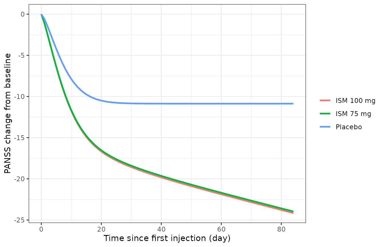
Typical change from baseline in PANSS for a US patient with baseline 95 and a gluteal injection.
PANSS model: virtual PRISMA-3 cohort
The virtual cohort has 200 patients per arm in each country (USA and
Ukraine). Baseline PANSS is drawn from a normal distribution with the
Table 1 mean (96.3) and coefficient of variation (8.3%), truncated to
the 80-120 entry range. All patients receive gluteal injections except
in the injection-site comparison below. CAV is the arm’s
typical value; the paper used each patient’s post hoc CL/F, whose
distribution it does not report.
set.seed(20250325)
rxode2::rxSetSeed(20250325)
n_per <- 200L
visits <- c(0, 4, 8, 15, 29, 57, 85)

make_cohort <- function(arm, region_usa, injsite_arm, id_offset) {
  bl <- round(pmin(pmax(rnorm(n_per, 96.3, 0.083 * 96.3), 80), 120))
  tibble::tibble(
    id = id_offset + seq_len(n_per),
    arm = arm,
    country = ifelse(region_usa == 1, "USA", "Ukraine"),
    site = ifelse(injsite_arm == 1, "Deltoid", "Gluteus"),
    CAV = unname(cav_arm[arm]),
    PANSS_BL = bl,
    REGION_USA = region_usa,
    INJSITE_ARM = injsite_arm,
    u_drop = runif(n_per)
  )
}

design <- tidyr::expand_grid(
  arm = names(cav_arm), region_usa = c(1, 0), injsite_arm = 0
) |>
  bind_rows(tibble::tibble(arm = names(cav_arm), region_usa = 1, injsite_arm = 1))
subj <- bind_rows(lapply(seq_len(nrow(design)), function(i) {
  make_cohort(design$arm[i], design$region_usa[i], design$injsite_arm[i], (i - 1L) * n_per)
}))
stopifnot(!anyDuplicated(subj$id))

ev <- tidyr::expand_grid(id = subj$id, time = sort(unique(c(0:85, visits)))) |>
  left_join(select(subj, id, CAV, PANSS_BL, REGION_USA, INJSITE_ARM), by = "id") |>
  mutate(evid = 0L)

sim <- rxode2::rxSolve(ui_panss, ev, returnType = "data.frame") |>
  left_join(select(subj, id, arm, country, site, u_drop), by = "id")
The dropout model of Appendix S1 gives each patient a survival curve
sur(t). A patient drops out at the first time
sur(t) falls below a uniform random number; visits after
dropout carry the last observed PANSS forward (LOCF), as in the paper’s
simulations.
drop_time <- sim |>
  group_by(id) |>
  summarise(t_drop = suppressWarnings(min(time[sur < u_drop[1]])), .groups = "drop")

vis <- sim |>
  filter(time %in% visits) |>
  left_join(drop_time, by = "id") |>
  arrange(id, time) |>
  group_by(id) |>
  mutate(
    y = ifelse(time < t_drop, sim, NA_real_),
    y_locf = y
  ) |>
  tidyr::fill(y_locf, .direction = "down") |>
  mutate(cfb = y_locf - y_locf[time == 0]) |>
  ungroup()

vis |>
  filter(site == "Gluteus") |>
  group_by(arm, country) |>
  summarise(`Dropped out by day 85 (%)` = round(100 * mean(is.na(y[time == 85])), 1), .groups = "drop") |>
knitr::kable(caption = "Simulated dropout by day 85 (gluteal cohorts).")| arm | country | Dropped out by day 85 (%) |
|---|---|---|
| ISM 100 mg | USA | 30.5 |
| ISM 100 mg | Ukraine | 23.5 |
| ISM 75 mg | USA | 33.5 |
| ISM 75 mg | Ukraine | 22.5 |
| Placebo | USA | 39.0 |
| Placebo | Ukraine | 24.5 |
Patients enrolled in the USA, and those with higher PANSS, drop out faster, which is why placebo patients drop out more often than actively treated ones.
Replicates Figure 1 (VPC by country and treatment)
vpc <- sim |>
  filter(site == "Gluteus", time %in% visits) |>
  group_by(arm, country, time) |>
  summarise(
    p05 = quantile(sim, 0.05), p50 = median(sim), p95 = quantile(sim, 0.95),
    .groups = "drop"
  )
ggplot(vpc, aes(time)) +
  geom_ribbon(aes(ymin = p05, ymax = p95), fill = "darkseagreen", alpha = 0.4) +
  geom_line(aes(y = p50), colour = "darkred", linewidth = 1) +
  facet_grid(country ~ factor(arm, levels = names(cav_arm))) +
  labs(x = "Time (day)", y = "PANSS") +
  theme_bw()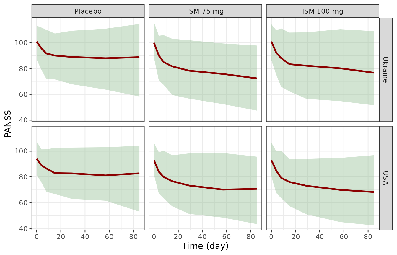
Simulated 5th, 50th and 95th percentiles of PANSS without dropout, by country and arm. Compare with Figure 1 of Lindauer 2025.
The observed medians in Figure 1 start near 100 in Ukraine and near 92 in the USA and, by day 85, fall to roughly 87 (placebo), 71 (75 mg) and 67 (100 mg) in Ukraine and 79, 66 and 69 in the USA (read from the figure). The model’s medians are compared below; Figure 1’s observed medians are of the patients still in the study, so they are not adjusted for dropout.
vpc |>
  filter(time %in% c(0, 85)) |>
  mutate(time = paste("Day", time)) |>
  select(arm, country, time, p50) |>
  tidyr::pivot_wider(names_from = time, values_from = p50) |>
  mutate(`Figure 1 day 85 (approx.)` = c(79, 87, 66, 71, 69, 67)[match(
    paste(arm, country),
    c(
      "Placebo USA", "Placebo Ukraine", "ISM 75 mg USA", "ISM 75 mg Ukraine",
      "ISM 100 mg USA", "ISM 100 mg Ukraine"
    )
  )]) |>
  mutate(across(where(is.numeric), ~ round(.x, 1))) |>
knitr::kable(caption = "Simulated median PANSS against the observed medians read from Figure 1.")| arm | country | Day 0 | Day 85 | Figure 1 day 85 (approx.) |
|---|---|---|---|---|
| ISM 100 mg | USA | 93.0 | 68.3 | 69 |
| ISM 100 mg | Ukraine | 100.9 | 76.7 | 67 |
| ISM 75 mg | USA | 92.8 | 70.7 | 66 |
| ISM 75 mg | Ukraine | 99.9 | 72.3 | 71 |
| Placebo | USA | 93.9 | 82.8 | 79 |
| Placebo | Ukraine | 100.7 | 88.8 | 87 |
Replicates Figure 2 (injection site, US patients)
fig2 <- vis |>
  filter(country == "USA", time <= 29) |>
  group_by(arm, site, time) |>
  summarise(
    p05 = quantile(cfb, 0.05), p50 = median(cfb), p95 = quantile(cfb, 0.95),
    .groups = "drop"
  )
ggplot(fig2, aes(time, p50, colour = site, fill = site)) +
  geom_ribbon(aes(ymin = p05, ymax = p95), alpha = 0.25, colour = NA) +
  geom_line(linewidth = 1) +
  facet_wrap(~ factor(arm, levels = names(cav_arm))) +
  labs(x = "Time (day)", y = "PANSS change from baseline", colour = "Injection site", fill = "Injection site") +
  theme_bw()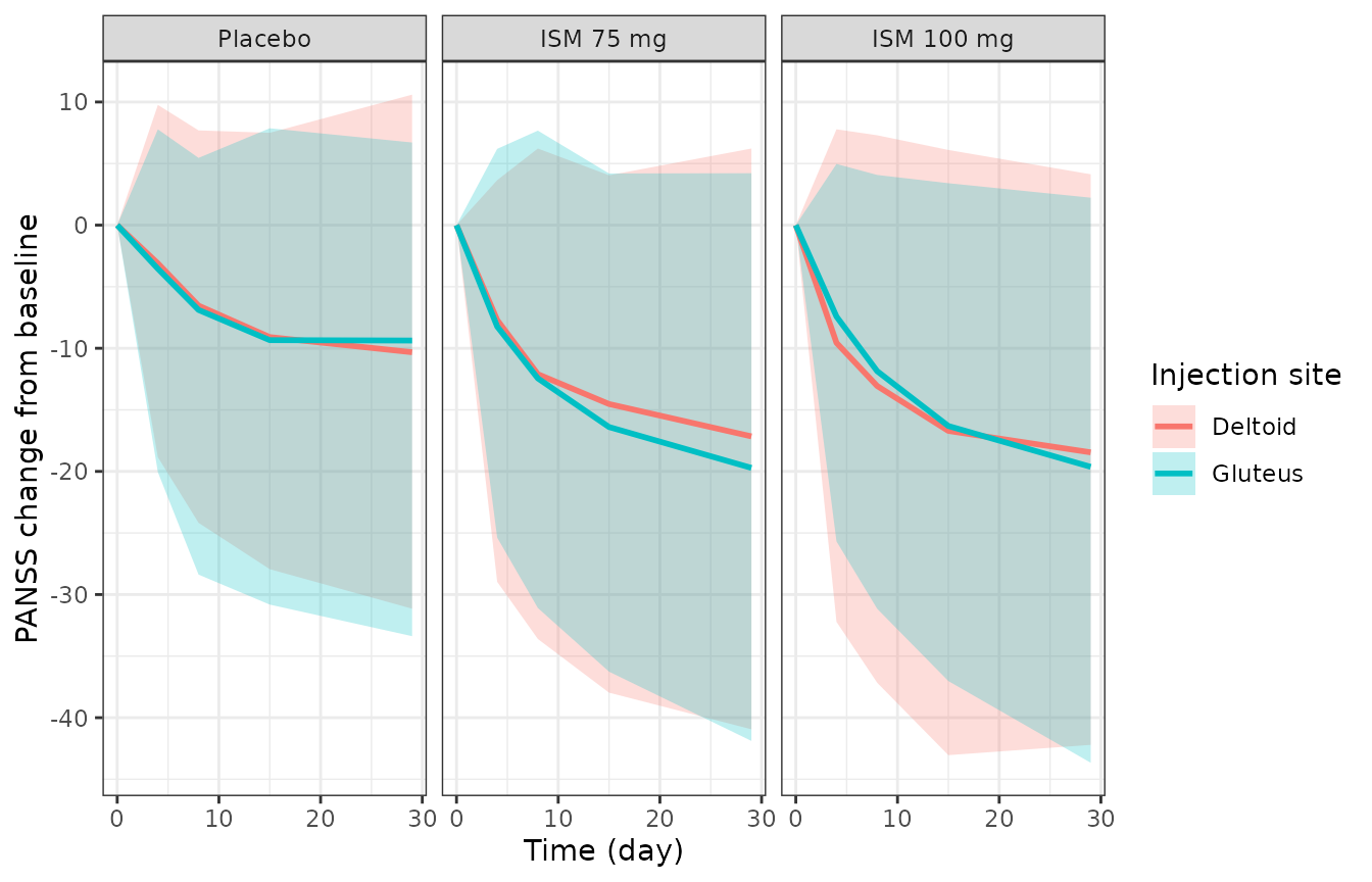
Median and 90% prediction interval of the PANSS change from baseline over the first 28 days in US patients by injection site, with dropout and LOCF. Compare with Figure 2 of Lindauer 2025.
In Figure 2 the median change at day 28 is about -10.5 points for placebo and about -18 points for both doses, with the deltoid curves slightly ahead of the gluteal ones in the first two weeks.
fig2_d29 <- fig2 |>
  filter(time == 29, site == "Gluteus") |>
  mutate(paper = c(Placebo = -10.5, `ISM 75 mg` = -18, `ISM 100 mg` = -17.5)[arm])
knitr::kable(
  fig2_d29 |>
    select(arm, p50, paper) |>
    mutate(p50 = round(p50, 1)) |>
    dplyr::rename(Arm = arm, `Simulated median` = p50, `Figure 2 (approx.)` = paper),
  caption = "Median PANSS change from baseline at the day-29 visit, US gluteal patients."
)| Arm | Simulated median | Figure 2 (approx.) |
|---|---|---|
| ISM 100 mg | -19.6 | -17.5 |
| ISM 75 mg | -19.7 | -18.0 |
| Placebo | -9.4 | -10.5 |
D2 receptor occupancy at the Risperidone ISM average concentration
The Uchida 2011 Emax model (Emax 100%, EC50 8.2 ng/mL), evaluated at the reported steady-state average active-moiety concentration of 38.6 ng/mL after 100 mg, gives an average occupancy of 82.5%. The full time course after each injection requires the Laveille 2024 Risperidone ISM population PK model.
Oral risperidone PK and D2 receptor occupancy
Replicates Figure S5
Figure S5 shows the active-moiety concentration and D2RO over the
first week of 3 and 4 mg once-daily oral risperidone in 1000 simulated
patients. Here 200 patients per dose are simulated, with CYP2D6
phenotype drawn from the mixture probabilities (4.93% poor, 8.26%
intermediate, 86.81% extensive metabolizers) and a new inter-occasion
draw for every dose (OCC = dose number).
set.seed(20250326)
rxode2::rxSetSeed(20250326)
n_oral <- 200L
obs_t <- sort(unique(c(seq(0, 168, by = 1), seq(0, 168, by = 0.25)[seq(0, 168, by = 0.25) < 6])))

oral_subj <- tidyr::expand_grid(dose = c(3, 4), k = seq_len(n_oral)) |>
  mutate(
    id = seq_len(n()),
    treatment = paste(dose, "mg QD"),
    phen = sample(c("PM", "IM", "EM"), n(), replace = TRUE, prob = c(0.0493, 0.0826, 0.8681)),
    CYP2D6_PM = as.integer(phen == "PM"),
    CYP2D6_IM = as.integer(phen == "IM")
  )

oral_ev <- bind_rows(
  tidyr::expand_grid(id = oral_subj$id, time = seq(0, 144, by = 24)) |>
    mutate(evid = 1L, cmt = "depot", dvid = NA_integer_),
  tidyr::expand_grid(id = oral_subj$id, time = obs_t) |>
    mutate(evid = 0L, cmt = NA_character_, dvid = 1L)
) |>
  left_join(select(oral_subj, id, dose, treatment, CYP2D6_PM, CYP2D6_IM), by = "id") |>
  mutate(
    amt = ifelse(evid == 1L, dose, 0),
    OCC = pmin(floor(time / 24) + 1, 7)
  ) |>
  arrange(id, time, desc(evid))

oral_sim <- rxode2::rxSolve(
  ui_oral, oral_ev,
  returnType = "data.frame", keep = "treatment"
)
s5 <- oral_sim |>
  select(id, time, treatment, AM, D2RO) |>
  tidyr::pivot_longer(c(AM, D2RO), names_to = "output") |>
  group_by(treatment, output, time) |>
  summarise(p05 = quantile(value, 0.05), p50 = median(value), p95 = quantile(value, 0.95), .groups = "drop")
ggplot(s5, aes(time, p50, colour = output, fill = output)) +
  geom_ribbon(aes(ymin = p05, ymax = p95), alpha = 0.2, colour = NA) +
  geom_line(linewidth = 0.8) +
  geom_hline(yintercept = 65, linetype = "dashed", colour = "red") +
  facet_wrap(~treatment, ncol = 1) +
  scale_colour_manual(values = c(AM = "darkorange", D2RO = "navy"), labels = c("Active moiety (ng/mL)", "D2RO (%)")) +
  scale_fill_manual(values = c(AM = "darkorange", D2RO = "navy"), labels = c("Active moiety (ng/mL)", "D2RO (%)")) +
  scale_x_continuous(breaks = seq(0, 168, by = 24)) +
  labs(x = "Time after first dose (h)", y = "Concentration (ng/mL) or D2RO (%)", colour = NULL, fill = NULL) +
  theme_bw()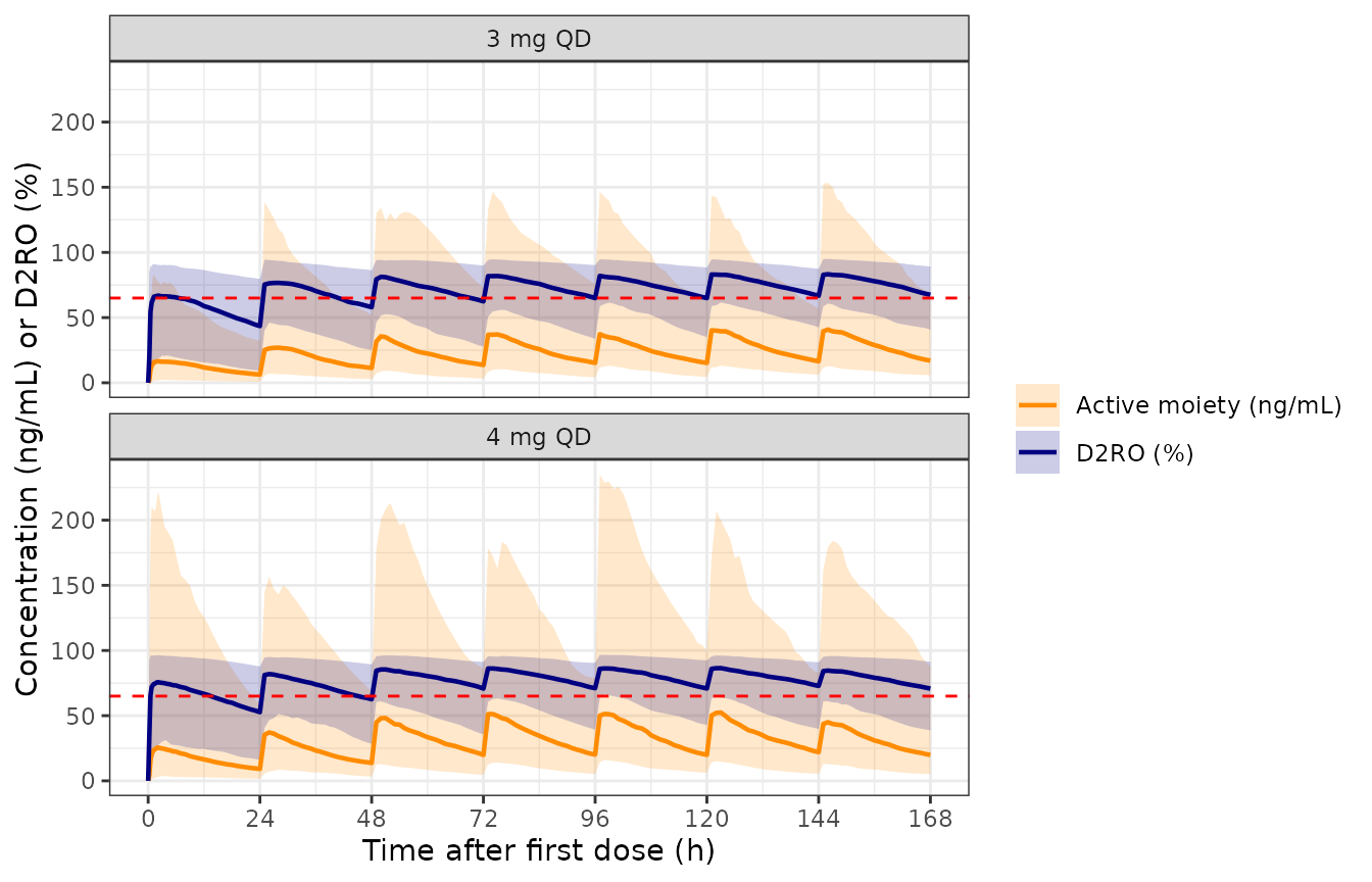
Median and 5th-95th percentiles of the active-moiety concentration (orange) and D2RO (blue) over the first week of oral risperidone. The dashed line marks 65% D2RO. Compare with Figure S5 of Lindauer 2025.
PKNCA of the active moiety
PKNCA is run on the active moiety for the first dosing interval and for the seventh (steady-state) interval, grouped by dose.
conc <- oral_sim |>
  filter(!is.na(AM)) |>
  select(id, time, treatment, AM) |>
  dplyr::rename(Cc = AM)
doses <- oral_ev |>
  filter(evid == 1L) |>
  select(id, time, treatment, amt)

conc_obj <- PKNCA::PKNCAconc(conc, Cc ~ time | treatment + id)
dose_obj <- PKNCA::PKNCAdose(doses, amt ~ time | treatment + id)
intervals <- data.frame(
  start = c(0, 144), end = c(24, 168),
  cmax = TRUE, tmax = TRUE, cmin = TRUE, cav = TRUE, auclast = TRUE
)
nca_res <- PKNCA::pk.nca(PKNCA::PKNCAdata(conc_obj, dose_obj, intervals = intervals))

nca_tbl <- as.data.frame(nca_res) |>
  filter(PPTESTCD %in% c("cmax", "tmax", "cmin", "cav")) |>
  mutate(interval = ifelse(start == 0, "Dose 1", "Dose 7")) |>
  group_by(treatment, interval, PPTESTCD) |>
  summarise(median = signif(median(PPORRES), 3), .groups = "drop") |>
  tidyr::pivot_wider(names_from = PPTESTCD, values_from = median)
nca_tbl |>
  dplyr::rename(
    Treatment = treatment, Interval = interval, `Cmax (ng/mL)` = cmax,
    `Tmax (h)` = tmax, `Cmin (ng/mL)` = cmin, `Cav (ng/mL)` = cav
  ) |>
knitr::kable(caption = "Median active-moiety NCA by dose and dosing interval.")| Treatment | Interval | Cav (ng/mL) | Cmax (ng/mL) | Cmin (ng/mL) | Tmax (h) |
|---|---|---|---|---|---|
| 3 mg QD | Dose 1 | 12.4 | 20.8 | 0.0 | 1.5 |
| 3 mg QD | Dose 7 | 29.4 | 43.9 | 13.3 | 1.0 |
| 4 mg QD | Dose 1 | 17.7 | 28.9 | 0.0 | 1.5 |
| 4 mg QD | Dose 7 | 32.1 | 47.9 | 15.8 | 1.0 |
The paper prints no NCA table for the oral comparator. Its median curves in Figure S5, read from the figure, give the reference below: first-dose peaks of about 19.5 and 25.5 ng/mL and seventh-dose peaks of about 38 and 49.5 ng/mL, with trough values of about 19 and 25 ng/mL at 168 h. The comparison pools the per-subject values by their median.
dose7 <- as.data.frame(nca_res) |>
  filter(start == 144, PPTESTCD %in% c("cmax", "cmin"))
published <- data.frame(
  treatment = c("3 mg QD", "4 mg QD"),
  cmax = c(38, 49.5),
  cmin = c(19, 25)
)
cmp <- nlmixr2lib::ncaComparisonTable(
  simulated = dose7,
  reference = published,
  by = "treatment",
  units = c(cmax = "ng/mL", cmin = "ng/mL"),
  tolerance_pct = 20
)
knitr::kable(cmp, caption = "Seventh-dose median active-moiety Cmax and Cmin against the medians read from Figure S5. * marks rows differing by more than 20%.")| NCA parameter | treatment | Reference | Simulated | % diff |
|---|---|---|---|---|
| Cmax (ng/mL) | 3 mg QD | 38 | 43.9 | +15.6% |
| Cmax (ng/mL) | 4 mg QD | 49.5 | 47.9 | -3.1% |
| Cmin (ng/mL) | 3 mg QD | 19 | 13.3 | -29.8%* |
| Cmin (ng/mL) | 4 mg QD | 25 | 15.8 | -37.0%* |
first_peak <- s5 |>
  filter(output == "AM", time <= 24) |>
  group_by(treatment) |>
  summarise(peak = max(p50), .groups = "drop") |>
  mutate(paper = c(`3 mg QD` = 19.5, `4 mg QD` = 25.5)[treatment])
t65 <- s5 |>
  filter(output == "D2RO", p50 >= 65) |>
  group_by(treatment) |>
  summarise(t65 = min(time), .groups = "drop")
knitr::kable(
  left_join(first_peak, t65, by = "treatment") |>
    mutate(peak = round(peak, 1)) |>
    dplyr::rename(
      Treatment = treatment, `Simulated first-dose median peak (ng/mL)` = peak,
      `Figure S5 (approx.)` = paper, `Median D2RO reaches 65% (h)` = t65
    ),
  caption = "First-dose median active-moiety peak and time for the median D2RO to reach 65%."
)| Treatment | Simulated first-dose median peak (ng/mL) | Figure S5 (approx.) | Median D2RO reaches 65% (h) |
|---|---|---|---|
| 3 mg QD | 16.6 | 19.5 | 1.25 |
| 4 mg QD | 25.6 | 25.5 | 0.50 |
# The PK is linear in dose, so the two arms differ only by a scale factor.
# Pooling their dose-normalised first-dose curves doubles the cohort behind
# the median: with 149% CV on KA and 158% IOV on D1, the median peak of one
# 200-patient arm moves by about 10% between rxode2 builds (16.6 vs 25.6 /
# 4 x 3 = 19.2 ng/mL for the 3 mg arm in one draw).
dose_by_id <- select(oral_subj, id, dose)
pooled_peak <- oral_sim |>
  filter(time <= 24) |>
  left_join(dose_by_id, by = "id") |>
  group_by(time) |>
  summarise(p50 = median(AM / dose), .groups = "drop") |>
  summarise(peak = max(p50)) |>
  dplyr::pull(peak)
paper_per_mg <- mean(c(19.5 / 3, 25.5 / 4))
cat(sprintf(
  "Pooled dose-normalised first-dose median peak: %.2f ng/mL per mg (Figure S5: %.2f)\n",
  pooled_peak, paper_per_mg
))
#> Pooled dose-normalised first-dose median peak: 6.06 ng/mL per mg (Figure S5: 6.44)
stopifnot(
  abs(pooled_peak - paper_per_mg) / paper_per_mg < 0.15,
  all(t65$t65 <= 3)
)
The first-dose peak, pooled over both doses after dose normalisation, is within about 10% of Figure S5, and the median D2RO passes 65% within the first one to two hours, as in the figure. The troughs, and the accumulation over the week, are lower than in Figure S5: the median concentration falls by about a factor of three between the first-dose peak and 24 h in this implementation and by about a factor of two in the figure. The typical extensive metabolizer reproduces the same faster decline, so the gap is not a matter of the inter-individual variability. No parameter in the Appendix S2 table, read as printed, closes it, and the values were not adjusted.
Assumptions and deviations
-
Exposure driver. The Methods define the Emax driver
as the average steady-state active-moiety concentration Cav,ss = Dose /
(CL/F x 28 days), computed per sampling occasion from the Laveille 2024
model; the control stream’s
$INPUTnames the columnCONC. The model takes it as theCAVcovariate (0 for placebo). The drift term, which the control stream switches on withIF(DOSE.NE.0), is switched on byCAV > 0; its random effect applies to every patient, as in the control stream. - Typical CAV in this vignette. The cohorts use one CAV per arm (38.6 ng/mL for 100 mg from the Discussion, scaled to 28.95 ng/mL for 75 mg) instead of individual post hoc values, which are not reported. Because EC50 (4.6 ng/mL) is far below both values, the PANSS predictions are insensitive to this.
- Time constant TD. Table 2 and the Results describe TD as the time to reach 68.3% of the maximal placebo effect. With the Weibull form, the fraction reached at t = TD is 1 - exp(-1) = 63.2% (the control-stream comment says 63%); the equation is implemented as printed.
- Drug-effect onset half-life. Table 2 and the control stream give KTHL in days (8.96 day); the Discussion’s “~9 h” is read as days.
- Dropout hazard sign. Appendix S1 prints h(t) = BHAZ x exp(-predictor x beta) with positive estimates beta_PANSS = 0.049 and beta_USA = 0.996. Read literally, a typical patient (PANSS about 90) would have a hazard near 1e-7 per day, so practically nobody would drop out, contradicting the stated purpose of the model (dropout depending on PANSS severity). The model therefore uses h = BHAZ x exp(0.049 x PANSS + 0.996 x USA): higher PANSS and US enrollment raise the hazard. PANSS enters uncentred and as the model-predicted individual score; the appendix does not say whether the observed or predicted score was used.
-
Country and injection site. PRISMA-3 enrolled only
in the USA and Ukraine, so the Ukraine effect on baseline is written
with
1 - REGION_USA. The deltoid indicatorINJSITE_ARMis the source’sSINJ - 1; the gluteal muscle is the reference. - IIV fixed to zero. The control stream carries zero-fixed variances for POW and EC50; those random effects are omitted.
-
Oral model: CYP2D6 phenotype. The source estimates
the phenotype as a latent three-subpopulation mixture. The model selects
the subpopulation through the indicators
CYP2D6_PMandCYP2D6_IM(extensive metabolizer when both are 0); this vignette draws them with the mixture probabilities. The single logit-scale IIV of FP and the single IIV of CLPM are shared by the three subpopulations, as the table prints one value for each. -
Oral model: IOV. The occasion is not defined in the
source. The model declares the inter-occasion random effects on F1, D1
and KA at the
OCClevel; this vignette draws a new value for every daily dose. - Oral model: active moiety. The active moiety is the plain sum of the risperidone and 9-hydroxyrisperidone concentrations (no molecular-weight correction is mentioned), and amounts converted to 9-hydroxyrisperidone are carried in risperidone mass units.
- Oral model: residual error. Not reported (the simulations exclude it); the proportional residual errors are fixed to 0.
- Oral model: trough discrepancy. See the PKNCA section: the simulated troughs and steady-state peaks are lower than those read from Figure S5.