Lecanemab population PK and ARIA-E exposure-response (Majid 2024)
Source:vignettes/articles/Majid_2024_lecanemab.Rmd
Majid_2024_lecanemab.RmdModel and source
Majid 2024 reports two fitted models, and this package ships them as two model files with one vignette (this page) covering the paper as a unit.
- Population PK: Majid O, Cao Y, Willis BA, Hayato S, Takenaka O, Lalovic B, Sreerama Reddy SH, Penner N, Reyderman L, Yasuda S, Hussein Z (2024). Population pharmacokinetics and exposure-response analyses of safety (ARIA-E and isolated ARIA-H) of lecanemab in subjects with early Alzheimer’s disease. CPT Pharmacometrics Syst Pharmacol. 2024;13(12):2111-2123. doi:10.1002/psp4.13224.
- ARIA-E exposure-response:
Majid_2024_lecanemab_ariae(same citation) - Article: https://doi.org/10.1002/psp4.13224
pk_mod   <- readModelDb("Majid_2024_lecanemab")
ariae_mod <- readModelDb("Majid_2024_lecanemab_ariae")
Population pharmacokinetics of the anti-amyloid-beta protofibril monoclonal antibody lecanemab (Leqembi) in 1619 subjects with early Alzheimer’s disease (mild cognitive impairment due to AD or mild AD dementia), from 21,929 serum concentrations pooled across two phase I studies (101, 104), the phase II study 201 Core and open-label extension, and the phase III Clarity AD study 301 Core and open-label extension. Linear two-compartment model with first-order elimination from the central compartment following a 1 h intravenous infusion, parameterized for CL, V1, V2 and Q. Covariate effects: body weight (power, reference 72 kg) and albumin (power, reference 43 g/L) on CL; female sex and sample-level ADA-positive status as multiplicative ratios on CL; body weight (power), female sex and Japanese race/ethnicity as ratios on V1; Japanese race/ethnicity as a ratio on V2. Q carries no covariate and no IIV. A manufacturing-process comparability factor F is applied to the intravenous dose: F is fixed at 1 for Process A and estimated at 0.904 for Process B, and the between-subject variability on F applies to Process B records ONLY (supplement Text S1 $PK codes it inside an IF (FORM.EQ.1) branch). CL and V1 IIV are correlated (R = 0.144). None of the retained covariates shifted steady-state AUC or Cmax outside the 0.8-1.25 acceptance interval, and age was not a significant covariate. The typical terminal half-life is 14.5 days. Companion exposure-response model: Majid_2024_lecanemab_ariae.
A third endpoint in the paper, isolated ARIA-H, was analysed graphically only and yielded no fitted model, so no model file exists for it. That is the paper’s own result rather than a transcription gap: Figure 4 shows the incidence of isolated ARIA-H against quartiles of Css,max, Css,av and Css,min with a linear smooth through each APOE4 genotype group and finds “little apparent correlation”, the rate being low (< 9%) and similar between placebo and lecanemab-treated subjects. The Results state explicitly that “based on these results, exposure relationship for isolated ARIA-H was not further explored with modeling approaches.”
Population
The population PK model was fit to 21,929 serum lecanemab concentrations from 1619 subjects with early Alzheimer’s disease pooled across four studies: two phase I studies (101 and 104), the phase II Study 201 Core and open-label extension, and the phase III Clarity AD Study 301 Core and open-label extension (NCT03887455). Baseline characteristics (Table S2): median age 72 years (range 50-93), median weight 72 kg (37.7-130.5), median albumin 43 g/L (35-54), 49.4% female, 80.7% White and 8.5% Japanese. Every lecanemab infusion in every contributing study ran over 60 +/- 10 minutes. Doses spanned 0.3-15 mg/kg as single doses and 2.5-10 mg/kg bi-weekly or monthly; 1113 of the 1619 subjects received the approved 10 mg/kg bi-weekly regimen. A total of 614 samples were excluded (BLQ, missing time, CWRES > 5, above 600 ug/mL, or time after dose over 2000 h).
The ARIA-E exposure-response analysis pooled 2641 subjects from Study 201 Core (852) and Study 301 Core (1789) – 1499 on lecanemab and 1142 on placebo – of whom 177 experienced ARIA-E. APOE4 genotype in that set was 803 non-carriers, 1423 heterozygous carriers and 415 homozygous carriers (Table S2).
The same information is available programmatically via each model’s
population metadata
(readModelDb("Majid_2024_lecanemab")()$population).
Source trace
Per-parameter provenance is recorded as an in-file comment beside
each ini() entry in
inst/modeldb/specificDrugs/Majid_2024_lecanemab.R and
inst/modeldb/specificDrugs/Majid_2024_lecanemab_ariae.R.
The table below collects them for review.
| Equation / parameter | Value | Source location |
|---|---|---|
lcl (CL) |
0.0154 L/h | Table 1, “CL (L/h)”; printed CL equation |
lvc (V1) |
3.24 L | Table 1, “V 1 (L)”; printed V1 equation |
lvp (V2) |
2.00 L | Table 1, “V 2 (L)”; printed V2 equation |
lq (Q) |
0.00718 L/h | Table 1, “Q (L/h)” |
lfcentral |
fixed log(1) | Supplement Text S1 $PK: F1=1 (Process A
anchor, no THETA) |
e_processb_f |
0.904 | Table 1, “F (comparability) for process B”; printed F equation |
e_wt_cl |
0.353 | Table 1, “Weight ~ CL (exponent)” |
e_alb_cl |
-0.374 | Table 1, “Albumin ~ CL (exponent)” |
e_female_cl |
0.791 | Table 1, “Females ~ CL (ratio to males)” |
e_ada_cl |
1.13 | Table 1, “ADApositive ~ CL (ratio to ADAnegative)” |
e_wt_vc |
0.513 | Table 1, “Weight ~ V 1 (exponent)” |
e_female_vc |
0.868 | Table 1, “Females ~ V 1 (ratio to males)” |
e_japanese_vc |
0.920 | Table 1, “Japanese ethnicity ~ V 1 (ratio to non-Japanese)” |
e_japanese_vp |
0.671 | Table 1, “Japanese ethnicity ~ V 2 (ratio to non-Japanese)” |
etalcl, etalvc block |
0.121801 / 0.006131 / 0.014884 | Table 1 IIV block (34.9%, R = 0.144, 12.2%); supplement Text S1
$OMEGA BLOCK(2)
|
etalvp |
0.894916 | Table 1 IIV block (94.6%) |
etalfcentral |
0.007242 | Table 1 IIV block (8.51%) |
propSd |
0.210 | Table 1, “Proportional (%CV)” 21.0 |
addSd |
1.12 ug/mL | Table 1, “Additive (SD; ug/mL)” |
| CL / V1 / V2 / F covariate equations | n/a | Printed equation block immediately below Table 1; confirmed
line-for-line by supplement Text S1 $PK
|
logit_ref (INT) |
-4.89 | Table 2, “Intercept (INT)” |
e_cmax_ariae (SLP) |
0.00666 per ug/mL | Table 2, “Slope of lecanemab exposure effect” |
e_apoe4_het_ariae |
0.640 | Table 2, “Cov APOE4 Hetero” |
e_apoe4_hom_ariae |
1.91 | Table 2, “Cov APOE4 Homo” |
| ARIA-E logit equation | n/a | Table 2 header row; supplement Text S2 $PRED
|
The IIV column of Table 1 is labelled “%CV”, but the table footnote
defines that column as “CV%, square root of variance x 100”. The printed
numbers are therefore omega standard deviations on the log scale, and
the usual omega^2 = log(CV^2 + 1) back-transform is
not applied; each variance is simply
(printed / 100)^2. This is the single most consequential
reading decision in the extraction and the footnote settles it
unambiguously.
Part 1 – Population PK
Virtual cohort
Original subject-level data are not public. The cohort below approximates the Study 301 population receiving the approved regimen: 10 mg/kg bi-weekly, Process B drug product, ADA-negative. Weight is drawn log-normally with median 72 kg and a spread chosen so the 5th / 95th percentiles land near the 49 and 99 kg values that the Figure 1 caption identifies as the 5th / 95th percentiles of the PK analysis set, then truncated to the observed 37.7-130.5 kg range. Albumin is drawn normally with median 43 g/L and a spread matched to the Figure 1 test values of 39 and 48 g/L, truncated to 35-54 g/L. Sex and Japanese ethnicity are drawn at the Table S2 marginal frequencies.
rxode2::rxSetSeed(20240001)
set.seed(20240001)

n_sub <- 200L          # per-arm cap
tau   <- 336           # bi-weekly, h
ndose <- 26L           # 1 year; terminal t1/2 is 348 h, so this is steady state
t_last <- tau * (ndose - 1L)

cohort <- tibble(
  id                = seq_len(n_sub),
  WT                = pmin(pmax(72 * exp(rnorm(n_sub, 0, 0.214)), 37.7), 130.5),
  ALB               = pmin(pmax(rnorm(n_sub, 43, 2.74), 35), 54),
  SEXF              = rbinom(n_sub, 1, 0.494),
  RACE_JAPANESE     = rbinom(n_sub, 1, 0.085),
  ADA_POS           = 0,
  FORM_LEC_PROCESSB = 1
)

dose_rows <- cohort |>
  mutate(amt = 10 * WT) |>
  expand_grid(time = tau * (0:(ndose - 1L))) |>
  mutate(evid = 1L, cmt = "central", dur = 1, dv = NA_real_)

obs_rows <- cohort |>
  expand_grid(time = t_last + seq(0, tau, by = 2)) |>
  mutate(evid = 0L, cmt = "central", amt = NA_real_, dur = NA_real_, dv = NA_real_)

events <- bind_rows(dose_rows, obs_rows) |> arrange(id, time, desc(evid))

cohort_sim <- rxode2::rxSolve(pk_mod, events, returnType = "data.frame") |>
  as_tibble() |>
  filter(!is.na(Cc))
#> ℹ parameter labels from comments will be replaced by 'label()'
Steady-state exposure versus the published values
The Discussion reports a PK-model-predicted mean Css,max of 305 ug/mL in subjects receiving 10 mg/kg bi-weekly in the phase III study, and gives the Study 301 predicted Css,max range as 58-544 ug/mL.
per_subject <- cohort_sim |>
  group_by(id) |>
  summarise(cmax = max(Cc), cmin = min(Cc), cav = mean(Cc), .groups = "drop")

exposure_chk <- tibble(
  quantity = c("Css,max mean (ug/mL)", "Css,max 5th pctile", "Css,max 95th pctile",
               "Css,min median", "Css,av median"),
  simulated = c(mean(per_subject$cmax),
                quantile(per_subject$cmax, 0.05),
                quantile(per_subject$cmax, 0.95),
                median(per_subject$cmin),
                median(per_subject$cav)),
  published = c(305, NA, NA, NA, NA)
) |>
  mutate(pct_diff = 100 * (simulated - published) / published)

knitr::kable(exposure_chk, digits = 1,
caption = "Simulated steady-state exposure vs the Majid 2024 Discussion")| quantity | simulated | published | pct_diff |
|---|---|---|---|
| Css,max mean (ug/mL) | 301.9 | 305 | -1 |
| Css,max 5th pctile | 205.7 | NA | NA |
| Css,max 95th pctile | 445.5 | NA | NA |
| Css,min median | 74.2 | NA | NA |
| Css,av median | 145.3 | NA | NA |
cmax_mean_pct <- 100 * (mean(per_subject$cmax) - 305) / 305

# Structural gate. A mis-transcribed clearance, volume, dose or unit would move
# the whole distribution by tens of percent. The centre is asserted, not the
# extremes (which are not reproducible across rxode2 builds).
stopifnot(abs(cmax_mean_pct) < 10)

# The simulated cohort should sit inside the paper's own predicted Study 301
# C(ss,max) range on a robust quantile basis rather than at the extremes.
stopifnot(
  quantile(per_subject$cmax, 0.05) > 58,
  quantile(per_subject$cmax, 0.95) < 544
)
The simulated cohort mean Css,max is 301.9 ug/mL against the published 305 ug/mL, a difference of -1.0%.
Typical subject: closed-form and terminal half-life gates
Two checks here have no stochastic component at all, so they are asserted tightly. Both sides of each comparison use the same fixed parameters, and the only difference is numerical integration error.
The reference subject is the one Figure 1 defines: 72 kg, male, non-Japanese, albumin 43 g/L, Process A drug product, all PK samples ADA-negative.
tv_mod <- rxode2::zeroRe(pk_mod)
#> ℹ parameter labels from comments will be replaced by 'label()'

tv_events <- bind_rows(
  tibble(time = tau * (0:(ndose - 1L)), evid = 1L, cmt = "central",
         amt = 720, dur = 1),
  # Final interval at steady state, then a long washout for the terminal slope.
  tibble(time = t_last + c(seq(0, tau, by = 1), seq(tau + 12, tau + 3500, by = 12)),
         evid = 0L, cmt = "central", amt = NA_real_, dur = NA_real_)
) |>
  mutate(id = 1L, WT = 72, ALB = 43, SEXF = 0, RACE_JAPANESE = 0,
         ADA_POS = 0, FORM_LEC_PROCESSB = 0, dv = NA_real_) |>
  arrange(time, desc(evid))

tv_sim <- rxode2::rxSolve(tv_mod, tv_events, returnType = "data.frame") |>
  as_tibble() |>
  filter(!is.na(Cc))
#> ℹ omega/sigma items treated as zero: 'etalcl', 'etalvc', 'etalvp', 'etalfcentral'

ss_window <- tv_sim |> filter(time >= t_last, time <= t_last + tau)

# Gate 1: average steady-state concentration against Dose * F / (CL * tau).
cav_sim <- mean(ss_window$Cc)
cav_cf  <- 720 * 1 / (0.0154 * tau)
cav_pct <- 100 * (cav_sim - cav_cf) / cav_cf
stopifnot(abs(cav_pct) < 0.5)

# Gate 2: terminal half-life from the Table 1 micro-constants against the
# Discussion's "approximately 14.5 days". Supplement Text S1 $PK computes T12
# by exactly this formula.
k10 <- 0.0154 / 3.24
k12 <- 0.00718 / 3.24
k21 <- 0.00718 / 2.00
s_sum <- k10 + k12 + k21
beta  <- 0.5 * (s_sum - sqrt(s_sum^2 - 4 * k21 * k10))
thalf_h <- log(2) / beta
stopifnot(abs(thalf_h / 24 - 14.5) < 0.1)

tibble(
  check = c("Css,av vs Dose*F/(CL*tau) (ug/mL)", "Terminal half-life (days)"),
  simulated = c(cav_sim, thalf_h / 24),
  reference = c(cav_cf, 14.5)
) |>
  mutate(pct_diff = 100 * (simulated - reference) / reference) |>
knitr::kable(digits = 3, caption = "Deterministic gates on the structural PK block")| check | simulated | reference | pct_diff |
|---|---|---|---|
| Css,av vs DoseF/(CLtau) (ug/mL) | 138.932 | 139.147 | -0.154 |
| Terminal half-life (days) | 14.501 | 14.500 | 0.007 |
ggplot(ss_window, aes(x = (time - t_last), y = Cc)) +
  geom_line(linewidth = 0.8) +
  labs(x = "Time after dose within the interval (h)",
       y = "Serum lecanemab (ug/mL)") +
  theme_bw()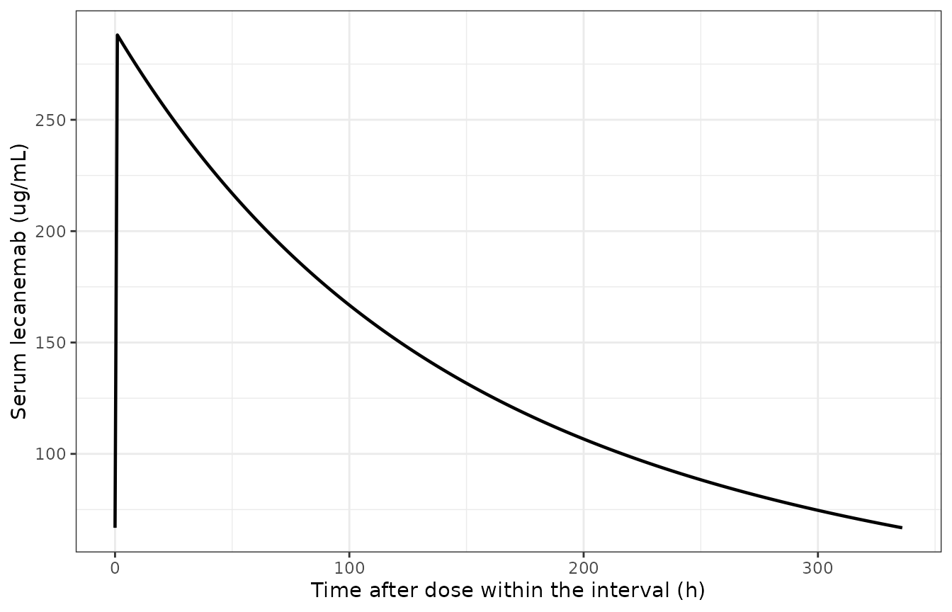
Typical-subject serum lecanemab over the final steady-state dosing interval, 10 mg/kg bi-weekly (reference subject, Process A).
Replicating Figure 1 – covariate forest plot
Replicates Figure 1 of Majid 2024, which plots the relative change in steady-state AUC and Cmax for each covariate against the reference subject, with a 0.80-1.25 acceptance interval shaded. Body weight is tested at 49 and 99 kg and albumin at 39 and 48 g/L (the 5th and 95th percentiles of the PK analysis set). Only the point estimates are reproduced here; the 90% CIs in Figure 1 come from 1000 draws from the final model’s variance-covariance matrix, which the paper does not publish.
scenarios <- tribble(
  ~covariate,          ~WT, ~ALB, ~SEXF, ~RACE_JAPANESE, ~ADA_POS, ~FORM_LEC_PROCESSB,
  "Reference",          72,   43,     0,              0,        0,                  0,
  "Weight 49 kg",       49,   43,     0,              0,        0,                  0,
  "Weight 99 kg",       99,   43,     0,              0,        0,                  0,
  "Albumin 39 g/L",     72,   39,     0,              0,        0,                  0,
  "Albumin 48 g/L",     72,   48,     0,              0,        0,                  0,
  "Female",             72,   43,     1,              0,        0,                  0,
  "ADA-positive",       72,   43,     0,              0,        1,                  0,
  "Japanese",           72,   43,     0,              1,        0,                  0,
  "Process B",          72,   43,     0,              0,        0,                  1
) |>
  mutate(id = row_number())

forest_events <- bind_rows(
  scenarios |> mutate(amt = 10 * WT) |>
    expand_grid(time = tau * (0:(ndose - 1L))) |>
    mutate(evid = 1L, cmt = "central", dur = 1),
  scenarios |>
    expand_grid(time = t_last + seq(0, tau, by = 1)) |>
    mutate(evid = 0L, cmt = "central", amt = NA_real_, dur = NA_real_)
) |>
  mutate(dv = NA_real_) |>
  arrange(id, time, desc(evid))

forest_sim <- rxode2::rxSolve(tv_mod, forest_events, returnType = "data.frame") |>
  as_tibble() |>
  filter(!is.na(Cc)) |>
  group_by(id) |>
  summarise(cmax = max(Cc), auc_tau = mean(Cc) * tau, .groups = "drop") |>
  left_join(scenarios |> select(id, covariate), by = "id")
#> ℹ omega/sigma items treated as zero: 'etalcl', 'etalvc', 'etalvp', 'etalfcentral'
#> Warning: multi-subject simulation without without 'omega'

ref_row <- forest_sim |> filter(covariate == "Reference")

forest <- forest_sim |>
  filter(covariate != "Reference") |>
  mutate(`AUCss ratio` = auc_tau / ref_row$auc_tau,
         `Cmax,ss ratio` = cmax / ref_row$cmax) |>
  select(covariate, `AUCss ratio`, `Cmax,ss ratio`)

knitr::kable(forest, digits = 3,
caption = "Figure 1 covariate effects on steady-state exposure, relative to the reference subject")| covariate | AUCss ratio | Cmax,ss ratio |
|---|---|---|
| Weight 49 kg | 0.780 | 0.815 |
| Weight 99 kg | 1.229 | 1.187 |
| Albumin 39 g/L | 0.964 | 0.986 |
| Albumin 48 g/L | 1.042 | 1.017 |
| Female | 1.264 | 1.204 |
| ADA-positive | 0.885 | 0.954 |
| Japanese | 1.000 | 1.052 |
| Process B | 0.904 | 0.904 |
forest |>
  pivot_longer(-covariate, names_to = "metric", values_to = "ratio") |>
  ggplot(aes(x = ratio, y = covariate, colour = metric)) +
  annotate("rect", xmin = 0.8, xmax = 1.25, ymin = -Inf, ymax = Inf,
           fill = "grey85", alpha = 0.6) +
  geom_vline(xintercept = 1, linetype = "dashed") +
  geom_point(size = 2.5, position = position_dodge(width = 0.4)) +
  scale_x_continuous(limits = c(0.6, 1.4)) +
  labs(x = "Ratio to reference subject", y = NULL, colour = NULL) +
  theme_bw() +
  theme(legend.position = "bottom")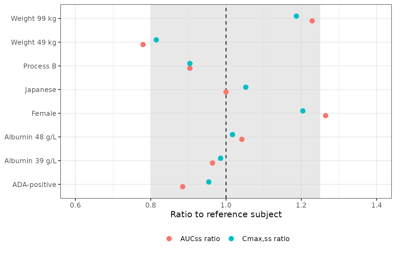
Replicates Figure 1 of Majid 2024: relative change in steady-state AUC and Cmax by covariate. Shaded band is the 0.80-1.25 acceptance interval.
Every covariate effect is small, reproducing the paper’s headline conclusion that no dose adjustment is warranted. Two point estimates sit marginally outside the 0.80-1.25 band – the 5th-percentile weight of 49 kg and female sex – which is consistent with the paper’s own wording that “CIs of all covariate effects were within or overlapped the reference 0.8-1.25 interval” (emphasis added). The paper asserts CI overlap, not point-estimate containment, so these rows are agreement rather than a discrepancy.
# All covariate effects must be modest. A sign error or a mis-read exponent
# would throw one of these well outside the band.
stopifnot(all(forest$`AUCss ratio` > 0.70), all(forest$`AUCss ratio` < 1.35))
# Directional gates fixed by the published coefficients: females and
# low-weight subjects have lower CL and hence higher AUC / lower AUC
# respectively; ADA-positive subjects clear faster; Process B gives less.
stopifnot(
  forest$`AUCss ratio`[forest$covariate == "Female"] > 1,
  forest$`AUCss ratio`[forest$covariate == "Weight 49 kg"] < 1,
  forest$`AUCss ratio`[forest$covariate == "ADA-positive"] < 1,
  abs(forest$`AUCss ratio`[forest$covariate == "Process B"] - 0.904) < 0.01
)
The Process B row reproduces the published comparability factor of 0.904 to three decimals, because relative bioavailability enters AUC exactly linearly.
Figure 2 of the paper is a prediction-corrected VPC stratified by study. It cannot be replicated here because it requires the observed concentrations, which are not public.
PKNCA validation
nca_conc <- cohort_sim |>
  filter(!is.na(Cc)) |>
  mutate(treatment = "Lecanemab 10 mg/kg Q2W (Process B)") |>
  select(id, time, Cc, treatment)

nca_dose <- cohort |>
  mutate(amt = 10 * WT,
         time = t_last,
         treatment = "Lecanemab 10 mg/kg Q2W (Process B)") |>
  select(id, time, amt, treatment)

conc_obj <- PKNCA::PKNCAconc(nca_conc, Cc ~ time | id / treatment)
dose_obj <- PKNCA::PKNCAdose(nca_dose, amt ~ time | treatment + id)

intervals <- data.frame(
  start = t_last, end = t_last + tau,
  cmax = TRUE, tmax = TRUE, cmin = TRUE, cav = TRUE, auclast = TRUE
)

nca_res <- PKNCA::pk.nca(PKNCA::PKNCAdata(conc_obj, dose_obj, intervals = intervals))
nca_out <- as.data.frame(nca_res)

knitr::kable(
  nca_out |>
    group_by(PPTESTCD) |>
    summarise(mean = mean(PPORRES), median = median(PPORRES),
              p5 = quantile(PPORRES, 0.05), p95 = quantile(PPORRES, 0.95),
              .groups = "drop"),
  digits = 1,
  caption = "PKNCA steady-state parameters over the final dosing interval (n = 200)"
)| PPTESTCD | mean | median | p5 | p95 |
|---|---|---|---|---|
| auclast | 52043.8 | 48985.0 | 25787.9 | 89765.4 |
| cav | 154.9 | 145.8 | 76.7 | 267.2 |
| cmax | 301.9 | 288.6 | 205.7 | 445.5 |
| cmin | 83.2 | 74.2 | 22.2 | 170.1 |
| tmax | 2.0 | 2.0 | 2.0 | 2.0 |
Comparison against published exposure metrics
Majid 2024 publishes no non-compartmental analysis table, so the reference column below carries the two absolute exposure quantities the paper does state: the mean Css,max of 305 ug/mL at 10 mg/kg bi-weekly (Discussion) and the typical-subject terminal half-life of 14.5 days = 348 h (Discussion). The simulated Css,max is aggregated with the mean to match the published statistic, and the half-life comes from the deterministic typical-subject arm, so both sides of each row are like-for-like.
simulated_nca <- tibble(
  PPTESTCD = c("cmax", "half.life"),
  PPORRES  = c(mean(nca_out$PPORRES[nca_out$PPTESTCD == "cmax"]), thalf_h)
)

reference_nca <- data.frame(cmax = 305, half.life = 348)

nca_tbl <- nlmixr2lib::ncaComparisonTable(
  simulated_nca, reference_nca,
  units = c(cmax = "ug/mL", half.life = "h")
)
knitr::kable(nca_tbl, caption = "Simulated vs published lecanemab exposure metrics")| NCA parameter | Reference | Simulated | % diff |
|---|---|---|---|
| Cmax (ug/mL) | 305 | 302 | -1.0% |
| t½ (h) | 348 | 348 | +0.0% |
attr(nca_tbl, "footnote")
#> NULL
Part 2 – ARIA-E exposure-response
The ARIA-E model is a static per-subject logistic regression with no
time dimension and no PK layer: exposure enters through the
CMAX covariate, which a user supplies as an individual
empirical-Bayes steady-state Cmaxin ug/mL
from the companion PK model. Placebo subjects enter at
CMAX = 0.
solve_ariae <- function(cmax, het = 0, hom = 0) {
  ev <- data.frame(id = seq_along(cmax), time = 0, amt = 0, evid = 0L,
                   CMAX = cmax, APOE4_HET = het, APOE4_HOM = hom)
  as.data.frame(
    rxode2::rxSolve(ariae_mod, ev, returnType = "data.frame")
  )$prob_ariae
}
odds <- function(p) p / (1 - p)
Audit of every published odds ratio
Table 2 prints an odds ratio alongside each coefficient, and the Discussion prints two more at the limits of the Study 301 exposure range. All five are reproduced from the shipped model by taking ratios of solved odds, so the audit exercises the model file rather than re-arithmetic on the table.
base_p <- solve_ariae(0)

or_audit <- tibble(
  quantity = c("Slope, per ug/dL (= 100 ug/mL)",
               "APOE4 heterozygous vs non-carrier",
               "APOE4 homozygous vs non-carrier",
               "Exposure at Css,max 58 ug/mL vs 0",
               "Exposure at Css,max 544 ug/mL vs 0"),
  simulated = c(odds(solve_ariae(100)) / odds(base_p),
                odds(solve_ariae(0, het = 1)) / odds(base_p),
                odds(solve_ariae(0, hom = 1)) / odds(base_p),
                odds(solve_ariae(58))  / odds(base_p),
                odds(solve_ariae(544)) / odds(base_p)),
  published = c(1.95, 1.90, 6.75, 1.47, 37.5)
) |>
  mutate(pct_diff = 100 * (simulated - published) / published)

knitr::kable(or_audit, digits = 3,
caption = "Every published ARIA-E odds ratio, recomputed from the shipped model")| quantity | simulated | published | pct_diff |
|---|---|---|---|
| Slope, per ug/dL (= 100 ug/mL) | 1.946 | 1.95 | -0.183 |
| APOE4 heterozygous vs non-carrier | 1.896 | 1.90 | -0.185 |
| APOE4 homozygous vs non-carrier | 6.753 | 6.75 | 0.046 |
| Exposure at Css,max 58 ug/mL vs 0 | 1.471 | 1.47 | 0.102 |
| Exposure at Css,max 544 ug/mL vs 0 | 37.451 | 37.50 | -0.130 |
Replicating the Figure 3 incidence anchors
The Discussion states that at the PK-model-predicted mean Css,max of 305 ug/mL in Study 301, ARIA-E incidence is predicted to be 28.0% (95% CI 22.6-34.1) in APOE4 homozygous carriers, 9.85% (7.96-12.1) in heterozygous carriers and 5.45% (3.75-7.84) in non-carriers. It also reports the observed Study 301 rates of 32.6%, 10.9% and 5.4%.
incidence <- tibble(
  genotype = c("Non-carrier", "Heterozygous", "Homozygous"),
  simulated_pct = 100 * c(solve_ariae(305),
                          solve_ariae(305, het = 1),
                          solve_ariae(305, hom = 1)),
  published_model_pct = c(5.45, 9.85, 28.0),
  observed_study301_pct = c(5.4, 10.9, 32.6)
) |>
  mutate(pct_diff_vs_model = 100 * (simulated_pct - published_model_pct) /
           published_model_pct)

knitr::kable(incidence, digits = 2,
caption = "Model-predicted ARIA-E incidence at Css,max = 305 ug/mL by APOE4 genotype")| genotype | simulated_pct | published_model_pct | observed_study301_pct | pct_diff_vs_model |
|---|---|---|---|---|
| Non-carrier | 5.42 | 5.45 | 5.4 | -0.49 |
| Heterozygous | 9.81 | 9.85 | 10.9 | -0.42 |
| Homozygous | 27.91 | 28.00 | 32.6 | -0.30 |
# Deterministic reproduction of the paper's own model predictions; the residual
# is the paper's 3-significant-figure rounding of the four coefficients.
stopifnot(all(abs(incidence$pct_diff_vs_model) < 1))
cmax_grid <- seq(0, 600, length.out = 200)

curves <- bind_rows(
  tibble(genotype = "Non-carrier",  cmax = cmax_grid, prob = solve_ariae(cmax_grid)),
  tibble(genotype = "Heterozygous", cmax = cmax_grid,
         prob = solve_ariae(cmax_grid, het = 1)),
  tibble(genotype = "Homozygous",   cmax = cmax_grid,
         prob = solve_ariae(cmax_grid, hom = 1))
) |>
  mutate(genotype = factor(genotype,
                           levels = c("Non-carrier", "Heterozygous", "Homozygous")))
#> Warning: multi-subject simulation without without 'omega'
#> Warning: multi-subject simulation without without 'omega'
#> Warning: multi-subject simulation without without 'omega'

ggplot(curves, aes(x = cmax, y = 100 * prob, colour = genotype)) +
  annotate("rect", xmin = 58, xmax = 544, ymin = -Inf, ymax = Inf,
           fill = "grey90", alpha = 0.6) +
  geom_vline(xintercept = 305, linetype = "dashed") +
  geom_line(linewidth = 0.9) +
  geom_point(
    data = incidence |>
      mutate(genotype = factor(genotype,
                               levels = c("Non-carrier", "Heterozygous", "Homozygous"))),
    aes(x = 305, y = published_model_pct, colour = genotype),
    shape = 21, fill = "white", size = 3, inherit.aes = FALSE,
    show.legend = FALSE
  ) +
  labs(x = "Model-predicted steady-state Cmax (ug/mL)",
       y = "Predicted ARIA-E incidence (%)", colour = "APOE4 genotype") +
  theme_bw() +
  theme(legend.position = "bottom")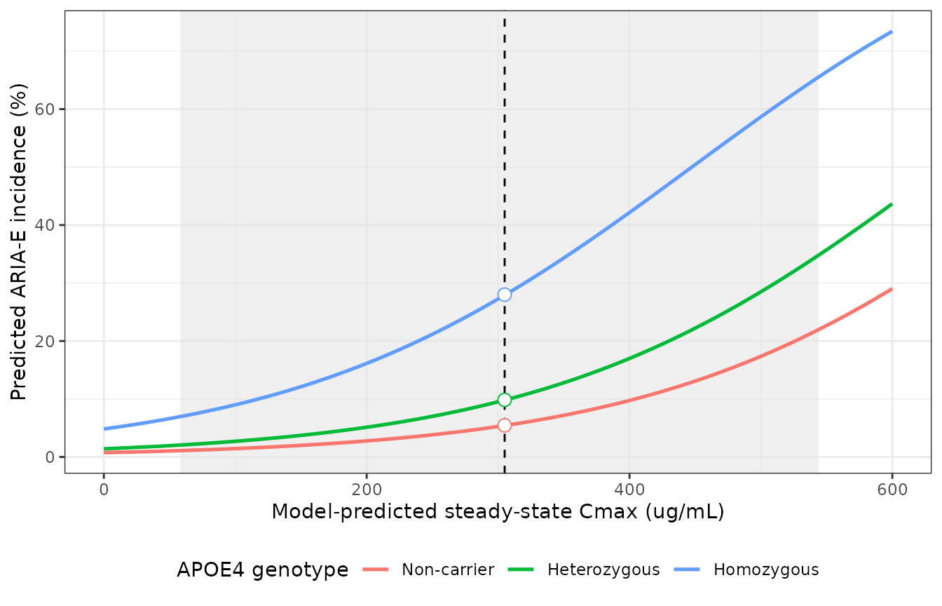
Replicates the top panel of Figure 3 of Majid 2024: model-predicted ARIA-E incidence versus steady-state Cmax by APOE4 genotype. Vertical line marks the Study 301 mean Css,max of 305 ug/mL; shaded band spans the paper’s predicted Study 301 Css,max range of 58-544 ug/mL.
Open circles are the three published point predictions at 305 ug/mL; the lines are the shipped model. They coincide.
End-to-end coupling: PK cohort into the ARIA-E model
The two models are designed to compose. Feeding each simulated subject’s own steady-state Cmax from Part 1 into the ARIA-E model, and assigning APOE4 genotype at the Table S2 frequencies (803 / 1423 / 415 of 2641), gives a cohort ARIA-E rate that can be compared with the observed Study 301 rates.
set.seed(20240002)
geno <- sample(c("Non-carrier", "Heterozygous", "Homozygous"),
               size = n_sub, replace = TRUE,
               prob = c(803, 1423, 415) / 2641)

coupled <- per_subject |>
  mutate(genotype = geno,
         APOE4_HET = as.integer(genotype == "Heterozygous"),
         APOE4_HOM = as.integer(genotype == "Homozygous"))

coupled$prob_ariae <- solve_ariae(coupled$cmax, coupled$APOE4_HET, coupled$APOE4_HOM)
#> Warning: multi-subject simulation without without 'omega'

coupled_summary <- coupled |>
  group_by(genotype) |>
  summarise(n = n(), mean_cmax = mean(cmax),
            mean_prob_pct = 100 * mean(prob_ariae), .groups = "drop") |>
  left_join(
    tibble(genotype = c("Non-carrier", "Heterozygous", "Homozygous"),
           observed_study301_pct = c(5.4, 10.9, 32.6)),
    by = "genotype"
  )

knitr::kable(coupled_summary, digits = 2,
caption = "PK cohort fed into the ARIA-E model, by APOE4 genotype, vs observed Study 301 rates")| genotype | n | mean_cmax | mean_prob_pct | observed_study301_pct |
|---|---|---|---|---|
| Heterozygous | 111 | 299.42 | 10.39 | 10.9 |
| Homozygous | 29 | 306.58 | 28.82 | 32.6 |
| Non-carrier | 60 | 304.34 | 6.10 | 5.4 |
# Ordering is structural: the homozygous coefficient is three times the
# heterozygous one, so the rank order cannot invert for any exposure.
ord <- coupled_summary |>
  arrange(match(genotype, c("Non-carrier", "Heterozygous", "Homozygous")))
stopifnot(all(diff(ord$mean_prob_pct) > 0))
# Overall cohort rate should land in a plausible band around the pooled
# observed Study 301 lecanemab-arm ARIA-E rate (12.6%, 129 of 1053 at
# 10 mg/kg Q2W per the Results).
stopifnot(100 * mean(coupled$prob_ariae) > 5,
          100 * mean(coupled$prob_ariae) < 25)
Assumptions and deviations
-
IIV scale. Table 1’s “%CV” column is read as omega
standard deviations x 100 because the table footnote defines it that way
(“CV%, square root of variance x 100”). The log-normal
omega^2 = log(CV^2 + 1)transform is deliberately not applied. If a future reader concludes the footnote is itself in error, everyetavariance in the model file would need revisiting; the point estimates and covariate effects would not. -
CL~V1 covariance. Table 1 publishes the IIV
correlation R = 0.144 rather than the covariance. The off-diagonal in
the model file is reconstructed as
R * omega_CL * omega_V1 = 0.144 * 0.349 * 0.122 = 0.006131, which is the only reading consistent with the printed$OMEGA BLOCK(2)structure. -
Bioavailability variability is Process-B-only.
Supplement Text S1
$PKcodesF1=1; IF (FORM.EQ.1) F1=THETA(5)*EXP(ETA(4)), so both the 0.904 ratio and its between-subject variability apply to Process B records only, and Process A bioavailability is exactly 1 with no variability. The model file reproduces that branch rather than putting the eta on a shared anchor. A reader who instead applied the eta to all records would inflate variability in the Process A studies. -
Residual error offset not reproduced. Supplement
Text S1
$ERRORisW = F + 0.01; Y = W + W*ERR(1) + ERR(2), in which the proportional term multiplies the prediction plus 0.01 ug/mL. The model file uses the standard nlmixr2prop() + add()form, which multiplies the prediction itself. The 0.01 ug/mL offset is a numerical guard sitting 50-fold below the 0.5 ug/mL assay LLOQ and has no practical effect on any simulation in this vignette. -
units$dosingis mg whileunits$concentrationis ug/mL. This is intentional and internally consistent: doses are in mg and volumes in L, so amount/volume is mg/L = ug/mL, and no scaling factor belongs inmodel().checkModelConventions()raises an informational note on the magnitude mismatch; the deterministicCss,avgate above confirms the arithmetic. - Virtual-cohort covariate distributions are assumed. The paper reports medians, ranges and 5th / 95th percentiles but not distributional forms, and no correlation structure beyond the qualitative note that weight is lower in females and in Asian subjects. The cohort here draws weight, albumin, sex and Japanese ethnicity independently, so it does not reproduce that correlation. Because all covariate effects are small this has little effect on the exposure summaries, but a user studying subgroup exposure should impose the correlation.
-
ADA and process held fixed in the cohort. The
virtual cohort is ADA-negative throughout and entirely Process B,
matching Study 301 Core. ADA status is genuinely time-varying at the
sample level in the source analysis; a user simulating seroconversion
should switch
ADA_POSfrom 0 to 1 partway through a subject’s record. -
Placeholder residual on the ARIA-E model. The
source fits a Bernoulli likelihood (
LAPLACE LIKEwith$OMEGA 0 FIX) and estimates no residual error and no random effect.addSd_prob_ariaeis a fixed 0.001 placeholder so rxode2 has an error model to attach to the typical-value probability; it is not a published quantity and must not be interpreted as one. - Figure 1 confidence intervals not reproduced. The 90% CIs in Figure 1 are generated from 1000 draws from the final model’s variance-covariance matrix, which the paper does not publish. Only the point estimates are replicated.
- Figure 2 (pcVPC) and Figure 4 (isolated ARIA-H) not reproduced. Both require the observed subject-level data, which are not public. Figure 4 in any case describes a graphical analysis that produced no model.
-
New canonical names registered with this
extraction.
FORM_LEC_PROCESSBwas added toinst/references/covariate-columns.mdas a member of the establishedFORM_<drug>_<feature>manufacturing-comparability family (siblingsFORM_LEB_NS0,FORM_SAR_DP2), andprob_ariaewas added toinst/references/compartment-names.mdas a member of the establishedprob_<endpoint>output family (siblingsprob_anemia,prob_hypertriglyceridemia,prob_dyskinesia).CMAXand theAPOE4_HET/APOE4_HOMpair were already canonical;Majid_2024_lecanemab_ariaewas added to theCMAXentry’s example-model list.
Errata and source gaps
No erratum or corrigendum for this article was located. The
supplement (Texts S1-S4, Tables S1-S7, Figures S1-S3) was retrieved and
is the source for the $PK and $PRED structural
confirmations cited above; note that the supplement’s
$THETA / $OMEGA / $SIGMA blocks
hold initial estimates only and were deliberately not
used as a parameter source. Every value in both model files comes from
Table 1, Table 2, the printed equation block below Table 1, or Table
S2.
One wording discrepancy is worth flagging because it inverts a sign if read carelessly: the Discussion says “Lecanemab clearance was found to decline with increasing albumin levels with an exponent of 0.374”, quoting the magnitude without the minus sign and carrying the direction in the verb. Table 1 and the printed CL equation both give -0.374, and that is what the model file uses.