modelName <- "Ma_2025_lenalidomide"
mod <- readModelDb(modelName)
ui <- rxode2::rxode(mod)
#> ℹ parameter labels from comments will be replaced by 'label()'
Model and source
- Citation: Ma Y, Song Z, Bing H, He H, Zhao L, Zhao R. Push Forward Clinical Management of Hematological Toxicity due to Lenalidomide Overexposure: Model-Informed Precision Dosing for Chinese Population With Renal Insufficiency. CPT Pharmacometrics Syst Pharmacol. 2025;14(7):1201-1210. doi:10.1002/psp4.70040
- Description: One-compartment oral population PK model with first-order absorption (Ka fixed) and first-order elimination for lenalidomide in Chinese adults with multiple myeloma or B-cell non-Hodgkin lymphoma, with Cockcroft-Gault creatinine clearance (power, centred at 94.2 mL/min) and fixed-exponent allometric body weight (centred at 63 kg) on CL/F and allometric body weight on V/F (Ma 2025)
- Article: https://doi.org/10.1002/psp4.70040
Ma 2025 developed a population PK model of oral lenalidomide in Chinese adults with multiple myeloma (MM) or B-cell non-Hodgkin lymphoma (NHL), sampled sparsely at steady state (one trough and one 1-h sample per patient), and used it for Monte Carlo dosing simulations across renal function. The structural model is one-compartment with first-order absorption and elimination. Because there was only one absorption-phase sample per patient, Ka was fixed to 8.34 1/h from Connarn 2018 and between-subject variability was estimated on CL/F only. Body weight enters CL/F and V/F with fixed allometric exponents (0.75 and 1.0, centred at the 63 kg median), and Cockcroft-Gault creatinine clearance (CCr) is the one covariate retained by the stepwise search, as a power effect on CL/F centred at the 94.2 mL/min median. Residual error is proportional.
The supplement (Data S1) gives the covariate-screening table (Table S1) and the Phoenix NLME model code. The code carries the base-model estimates (tvV = 37.61 L, residual 0.504, omega^2 = 0.032 with the CCr exponent disabled), so the final-model values below come from Table 3. No erratum or correction is indexed against the DOI (Europe PMC search, 2026-11-05).
Population
pop <- ui$population97 patients contributed 164 lenalidomide plasma concentrations in a multicentre prospective study at four Beijing hospitals (October 2021 to February 2022). Of these, 55 (56.7%) had MM and 42 (43.3%) B-cell NHL (DLBCL, FL, MCL, MZL, HGBL); 53 (54.6%) were women. Age was 33-87 years (median 62), weight 37-101 kg (median 63), and Cockcroft-Gault CCr 34.8-227.7 mL/min (median 94.2) (Ma 2025 Table 1). Doses were 10-25 mg once daily for 21 days of a 28-day cycle, 69.1% of patients at 25 mg. Patients had taken at least three doses before sampling.
The same information is available programmatically via
readModelDb("Ma_2025_lenalidomide")()$population.
Source trace
| Equation / parameter | Value | Source location |
|---|---|---|
lka (Ka) |
8.34 1/h, fixed | Table 3 tvKa (h-1) [17] = 8.34 (fixed); Results “PopPK
Modeling” (taken from Connarn 2018, reference 17) |
lcl (CL/F) |
7.4 L/h | Table 3 tvCL/F = 7.4 (5.66); bootstrap 6.74-8.24 |
lvc (V/F) |
37.4 L | Table 3 tvV/F = 37.4 (6.37); bootstrap 33.40-42.13 |
e_crcl_cl |
0.25 | Table 3 thetaCCr = 0.25 (30.88); bootstrap
0.14-0.34 |
e_wt_cl |
0.75, fixed | Table 3 CL/F equation; Methods “Base Structural Model”; supplement
Material IV dCldwt(freeze) = 0.75
|
e_wt_vc |
1, fixed | Table 3 V/F equation; supplement Material IV
dVdwt(freeze) = 1
|
etalcl |
omega^2 = 0.025 | Results text “a variance of 0.025”; Table 3
etaCL/F, %CV = 15.8
|
propSd |
0.495 | Table 3 RV, %CV = 49.5 (13.0)
|
| CL/F equation | 7.4 x (CCr/94.2)^0.25 x (WT/63)^0.75 x exp(eta) |
Results “PopPK Modeling” final expression; Table 3 |
| V/F equation | 37.4 x (WT/63)^1.0 |
Table 3 |
| One-compartment, first-order absorption | n/a | Results “PopPK Modeling”; supplement Material IV
cfMicro(A1, Cl / V, first = (Aa = Ka))
|
| Proportional residual error | n/a | Results “PopPK Modeling”; supplement Material IV
observe(CObs = C * (1 + CEps))
|
The Table 3 percentages for eta are omega itself, not the exact log-normal CV: 0.158^2 = 0.02496 matches the text’s 0.025, and the base-model 17.9% matches the supplement code’s omega^2 = 0.032 (sqrt = 0.179).
Deterministic checks
Ma 2025’s Discussion states that halving CCr lowers CL/F by about 15.9%, and its covariate equation gives CL/F = 7.4 L/h for the 63 kg, 94.2 mL/min reference subject. Both follow from the typical-value model with no randomness, so tight tolerances are correct here.
modTypical <- rxode2::zeroRe(mod)
#> ℹ parameter labels from comments will be replaced by 'label()'

typEvents <- data.frame(
  id = 1:2, time = 0, amt = NA_real_, evid = 0L, cmt = "central",
  WT = 63, CRCL = c(94.2, 94.2 / 2)
)
typ <- as.data.frame(rxode2::rxSolve(modTypical, events = typEvents))
#> ℹ omega/sigma items treated as zero: 'etalcl'
#> Warning: multi-subject simulation without without 'omega'

clRef <- typ$cl[typ$id == 1]
clHalf <- typ$cl[typ$id == 2]
pctDrop <- 100 * (1 - clHalf / clRef)
tHalfRef <- log(2) * typ$vc[1] / clRef

stopifnot(
  abs(clRef - 7.4) < 1e-6,
  abs(typ$vc[1] - 37.4) < 1e-6,
  abs(pctDrop - 15.9) < 0.05
)

data.frame(
  quantity = c(
    "CL/F, reference subject (L/h)",
    "CL/F reduction when CCr is halved (%)",
    "Terminal half-life, reference subject (h)"
  ),
  model = c(clRef, pctDrop, tHalfRef),
  paper = c("7.4 (Table 3)", "about 15.9 (Discussion)", "3-5 (Methods)")
) |>
  dplyr::rename("Quantity" = quantity, "Model" = model, "Ma 2025" = paper) |>
knitr::kable(digits = 2)| Quantity | Model | Ma 2025 |
|---|---|---|
| CL/F, reference subject (L/h) | 7.40 | 7.4 (Table 3) |
| CL/F reduction when CCr is halved (%) | 15.91 | about 15.9 (Discussion) |
| Terminal half-life, reference subject (h) | 3.50 | 3-5 (Methods) |
Virtual cohort for the dosing simulations
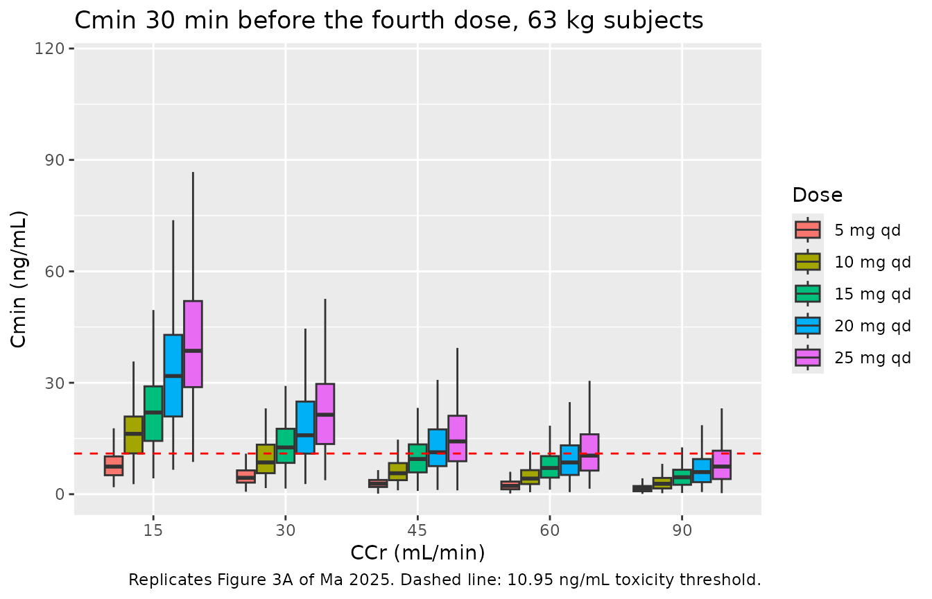
Ma 2025 does not state how body weight was handled in its Monte Carlo simulations. Every simulated subject here weighs 63 kg (the model’s reference weight) and the only random effect is the eta on CL/F, because that is what reproduces the published spread: the paper’s 25 mg interquartile range of AUC0-24h (3028.0-3729.6, about +/-10% around the median) matches the +/-0.674 x 0.158 = +/-10.6% expected from the CL/F eta alone, and would be about +/-14% if a weight distribution with the cohort’s SD of 11.7 kg were added. CCr is set to the fixed values on the x-axis of Ma 2025 Figure 3.
Residual error is not added: the paper’s simulated quantities are model concentrations, not simulated observations.
rxode2::rxSetSeed(20250701)

nPerArm <- 200L

# Cmin is read at 71.5 h, i.e. 30 min before the fourth once-daily dose
# (Ma 2025 Results "Model-Informed Precision Dosing"). The every-other-day arm
# is read at the same clock time, 23.5 h after its second dose; see the
# section on the every-other-day regimen below.
tCmin <- 71.5

arms <- dplyr::bind_rows(
  tidyr::crossing(
    CRCL = c(10, 15, 30, 45, 60, 90),
    dose = c(5, 10, 15, 20, 25),
    tau = 24
  ),
  tidyr::crossing(CRCL = c(10, 15, 30), dose = 15, tau = 48)
) |>
  dplyr::mutate(
    regimen = ifelse(tau == 24, paste0(dose, " mg qd"), paste0(dose, " mg qod")),
    arm = dplyr::row_number()
  )

subjects <- arms |>
  tidyr::crossing(rep = seq_len(nPerArm)) |>
  dplyr::mutate(id = dplyr::row_number(), WT = 63)

doseRows <- subjects |>
  dplyr::rowwise() |>
  dplyr::reframe(id, WT, CRCL, regimen, dose, time = seq(0, 48, by = tau)) |>
  dplyr::mutate(amt = dose, evid = 1L, cmt = "depot")
obsRows <- subjects |>
  dplyr::transmute(id, WT, CRCL, regimen, dose, time = tCmin, amt = NA_real_, evid = 0L, cmt = "central")

cminEvents <- dplyr::bind_rows(doseRows, obsRows) |>
  dplyr::arrange(id, time, dplyr::desc(evid)) |>
  dplyr::select(id, time, amt, evid, cmt, WT, CRCL, regimen, dose)

cmin <- rxode2::rxSolve(mod, events = cminEvents, keep = c("regimen", "dose")) |>
  as.data.frame() |>
  dplyr::filter(time == tCmin) |>
  dplyr::mutate(
    regimen = factor(regimen, levels = c(paste0(c(5, 10, 15, 20, 25), " mg qd"), "15 mg qod"))
  )
#> ℹ parameter labels from comments will be replaced by 'label()'
Replicating Figure 3: Cmin by renal function and dose
cmin |>
  dplyr::filter(CRCL %in% c(15, 30, 45, 60, 90), regimen != "15 mg qod") |>
  ggplot(aes(factor(CRCL), Cc, fill = regimen)) +
  geom_boxplot(outlier.shape = NA) +
  geom_hline(yintercept = 10.95, linetype = "dashed", colour = "red") +
  labs(
    x = "CCr (mL/min)", y = "Cmin (ng/mL)", fill = "Dose",
    title = "Cmin 30 min before the fourth dose, 63 kg subjects",
    caption = "Replicates Figure 3A of Ma 2025. Dashed line: 10.95 ng/mL toxicity threshold."
  )
cmin |>
  dplyr::filter(CRCL %in% c(10, 15, 30), regimen %in% c("5 mg qd", "10 mg qd", "15 mg qod")) |>
  ggplot(aes(factor(CRCL), Cc, fill = regimen)) +
  geom_boxplot(outlier.shape = NA) +
  geom_hline(yintercept = 10.95, linetype = "dashed", colour = "red") +
  labs(
    x = "CCr (mL/min)", y = "Cmin (ng/mL)", fill = "Dose",
    title = "Severe renal impairment",
    caption = "Replicates Figure 3B of Ma 2025."
  )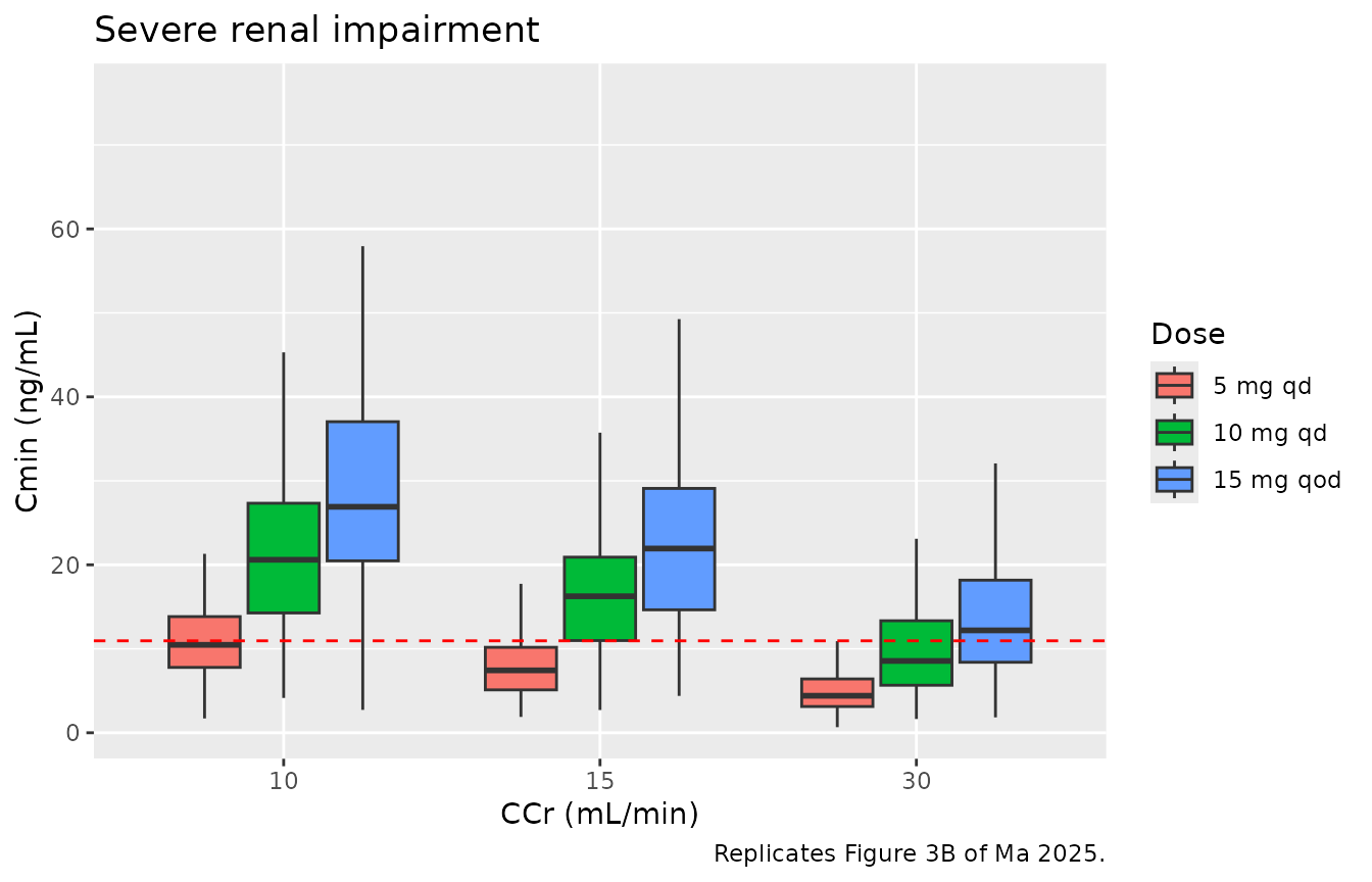
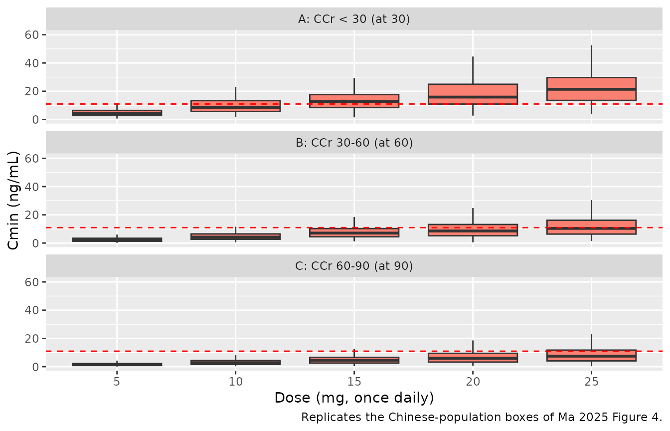
Ma 2025 reports several Figure 3B and Figure 4A statistics in the text. The figure 4 panels for the Chinese population line up with CCr = 30, 60 and 90 mL/min, the upper limit of each renal-function band (for example the CCr < 30 band’s 5 mg and 25 mg medians, 4.2 and 21.4 ng/mL, equal the CCr = 30 mL/min values here).
published <- tibble::tribble(
  ~CRCL, ~regimen,    ~statistic, ~published, ~source,
  10,    "5 mg qd",   "median",   9.9,        "Results, Fig 3B",
  10,    "5 mg qd",   "Q25",      7.1,        "Results, Fig 3B",
  10,    "5 mg qd",   "Q75",      13.3,       "Results, Fig 3B",
  30,    "15 mg qod", "median",   11.8,       "Results, Fig 3B",
  15,    "15 mg qod", "Q25",      15.5,       "Results, Fig 3B",
  30,    "10 mg qd",  "median",   8.2,        "Results, Fig 3B",
  15,    "10 mg qd",  "median",   11.1,       "Results, Fig 3B (see below)",
  30,    "5 mg qd",   "median",   4.2,        "Results, Fig 4A",
  30,    "25 mg qd",  "median",   21.4,       "Results, Fig 4A"
)

simStats <- cmin |>
  dplyr::mutate(regimen = as.character(regimen)) |>
  dplyr::group_by(CRCL, regimen) |>
  dplyr::summarise(
    median = median(Cc),
    Q25 = unname(quantile(Cc, 0.25)),
    Q75 = unname(quantile(Cc, 0.75)),
    .groups = "drop"
  ) |>
  tidyr::pivot_longer(c(median, Q25, Q75), names_to = "statistic", values_to = "simulated")

cminCheck <- published |>
  dplyr::left_join(simStats, by = c("CRCL", "regimen", "statistic")) |>
  dplyr::mutate(pct_diff = 100 * (simulated - published) / published)

cminCheck |>
  dplyr::select(CRCL, regimen, statistic, published, simulated, pct_diff, source) |>
  dplyr::rename(
    "CCr (mL/min)" = CRCL, "Regimen" = regimen, "Statistic" = statistic,
    "Ma 2025 (ng/mL)" = published, "Simulated (ng/mL)" = simulated,
    "Difference (%)" = pct_diff, "Source" = source
  ) |>
knitr::kable(digits = 1)| CCr (mL/min) | Regimen | Statistic | Ma 2025 (ng/mL) | Simulated (ng/mL) | Difference (%) | Source |
|---|---|---|---|---|---|---|
| 10 | 5 mg qd | median | 9.9 | 10.5 | 5.7 | Results, Fig 3B |
| 10 | 5 mg qd | Q25 | 7.1 | 7.8 | 9.6 | Results, Fig 3B |
| 10 | 5 mg qd | Q75 | 13.3 | 13.8 | 4.0 | Results, Fig 3B |
| 30 | 15 mg qod | median | 11.8 | 12.2 | 3.3 | Results, Fig 3B |
| 15 | 15 mg qod | Q25 | 15.5 | 14.6 | -5.5 | Results, Fig 3B |
| 30 | 10 mg qd | median | 8.2 | 8.6 | 4.3 | Results, Fig 3B |
| 15 | 10 mg qd | median | 11.1 | 16.3 | 46.4 | Results, Fig 3B (see below) |
| 30 | 5 mg qd | median | 4.2 | 4.4 | 4.9 | Results, Fig 4A |
| 30 | 25 mg qd | median | 21.4 | 21.4 | -0.1 | Results, Fig 4A |
# The CCr 15 / 10 mg qd row is excluded: the text value contradicts the
# paper's own Figure 3B (see below). For the rest, medians move with a
# mis-transcribed CL, exponent or dose by tens of percent, while the Monte Carlo
# error of a 200-subject median or quartile is a few percent.
gated <- cminCheck |> dplyr::filter(!(CRCL == 15 & regimen == "10 mg qd"))
stopifnot(
  nrow(gated) == 8L,
  abs(median(gated$pct_diff)) < 10,
  all(abs(gated$pct_diff[gated$statistic == "median"]) < 15),
  all(abs(gated$pct_diff) < 25)
)
Every gated statistic is reproduced within about 10%. The one row that does not match, CCr 15 mL/min at 10 mg once daily, is printed in the text as a median of 11.1 ng/mL, but Figure 3B of the same paper draws that box’s median at about 15 ng/mL with its lower quartile near 11, and the model’s typical value at that CCr and dose is about 15.1 ng/mL. The text value appears to be the lower quartile mislabelled as the median.
The every-other-day regimen
The paper defines Cmin as the concentration “30 min prior to the fourth dose following three consecutive doses”. Read literally for 15 mg every other day, that is 143.5 h, 47.5 h after the third dose, where the typical concentration is far below the published values. The published 15 mg every-other-day medians are reproduced only when the regimen is read at 23.5 h after a dose (here, at the same 71.5 h clock time as the once-daily arms):
qodEvents <- data.frame(
  id = c(1, 1, 1, 1, 2, 2, 2),
  time = c(0, 48, 96, 143.5, 0, 48, 71.5),
  amt = c(15, 15, 15, NA, 15, 15, NA),
  evid = c(1L, 1L, 1L, 0L, 1L, 1L, 0L),
  cmt = c("depot", "depot", "depot", "central", "depot", "depot", "central"),
  WT = 63, CRCL = 30
)
qod <- as.data.frame(rxode2::rxSolve(modTypical, events = qodEvents)) |>
  dplyr::filter(time %in% c(71.5, 143.5))
#> ℹ omega/sigma items treated as zero: 'etalcl'
#> Warning: multi-subject simulation without without 'omega'

data.frame(
  reading = c("47.5 h after the 3rd dose (literal)", "23.5 h after a dose"),
  Cc = qod$Cc[order(qod$time, decreasing = TRUE)]
) |>
  dplyr::rename("Sampling time" = reading, "Typical Cmin at CCr 30 (ng/mL)" = Cc) |>
knitr::kable(digits = 2, caption = "Ma 2025 reports a median of 11.8 ng/mL for this arm.")| Sampling time | Typical Cmin at CCr 30 (ng/mL) |
|---|---|
| 47.5 h after the 3rd dose (literal) | 0.35 |
| 23.5 h after a dose | 12.43 |
Replicating Figure 4 (Chinese arm)
Figure 4 also shows a predominantly non-Asian model (Hughes 2019), which is not part of this model file; only the Chinese arm is replicated.
cmin |>
  dplyr::filter(CRCL %in% c(30, 60, 90), regimen != "15 mg qod") |>
  dplyr::mutate(
    band = factor(
      CRCL,
      levels = c(30, 60, 90),
      labels = c("A: CCr < 30 (at 30)", "B: CCr 30-60 (at 60)", "C: CCr 60-90 (at 90)")
    )
  ) |>
  ggplot(aes(factor(dose), Cc)) +
  geom_boxplot(outlier.shape = NA, fill = "salmon") +
  geom_hline(yintercept = 10.95, linetype = "dashed", colour = "red") +
  facet_wrap(~band, ncol = 1) +
  labs(
    x = "Dose (mg, once daily)", y = "Cmin (ng/mL)",
    caption = "Replicates the Chinese-population boxes of Ma 2025 Figure 4."
  )
Replicating Figure 5 and NCA with PKNCA
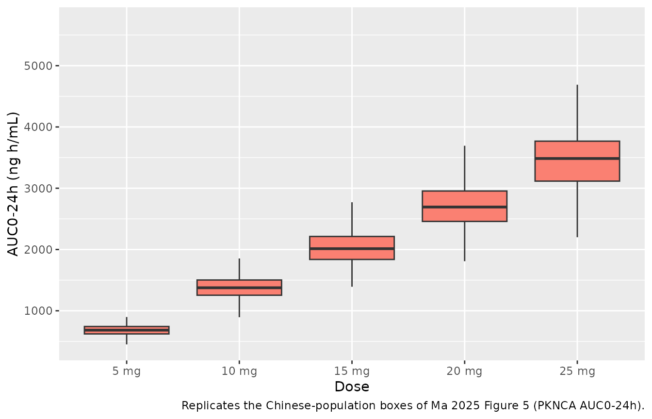
Figure 5 compares AUC0-24h after doses of 5-25 mg in patients with normal renal function (CCr = 90 mL/min). The paper’s AUC is “within the initial 24 h”, so a single dose is simulated and the AUC over 0-24 h is computed with PKNCA. The axis label in Ma 2025 reads “mg/L/h”, but the values (3376.7 at 25 mg, i.e. 25 mg / 7.3 L/h = 3.4 mg h/L) are in ng h/mL.
ncaSubjects <- tidyr::crossing(dose = c(5, 10, 15, 20, 25), rep = seq_len(nPerArm)) |>
  dplyr::mutate(id = dplyr::row_number(), WT = 63, CRCL = 90, treatment = paste0(dose, " mg"))

obsTimes <- c(seq(0, 2, by = 0.05), seq(2.25, 24, by = 0.25))
ncaEvents <- dplyr::bind_rows(
  ncaSubjects |> dplyr::mutate(time = 0, amt = dose, evid = 1L, cmt = "depot"),
  ncaSubjects |>
    tidyr::crossing(time = obsTimes) |>
    dplyr::mutate(amt = NA_real_, evid = 0L, cmt = "central")
) |>
  dplyr::arrange(id, time, dplyr::desc(evid)) |>
  dplyr::select(id, time, amt, evid, cmt, WT, CRCL, treatment, dose)

ncaSim <- rxode2::rxSolve(mod, events = ncaEvents, keep = c("treatment", "dose")) |>
  as.data.frame()
concData <- ncaSim |>
  dplyr::filter(!is.na(Cc)) |>
  dplyr::select(id, time, Cc, treatment)
doseData <- ncaSubjects |>
  dplyr::transmute(id, time = 0, amt = dose, treatment)

concObj <- PKNCA::PKNCAconc(concData, Cc ~ time | treatment + id)
doseObj <- PKNCA::PKNCAdose(doseData, amt ~ time | treatment + id)
intervals <- data.frame(start = 0, end = 24, cmax = TRUE, tmax = TRUE, auclast = TRUE)
ncaRes <- PKNCA::pk.nca(PKNCA::PKNCAdata(concObj, doseObj, intervals = intervals))

ncaTbl <- as.data.frame(ncaRes$result)
auc25 <- ncaTbl |> dplyr::filter(treatment == "25 mg", PPTESTCD == "auclast")
aucQ <- quantile(auc25$PPORRES, c(0.25, 0.5, 0.75))

reference <- data.frame(treatment = "25 mg", auclast = 3376.7)
cmp <- nlmixr2lib::ncaComparisonTable(
  ncaRes, reference,
  by = "treatment",
  units = c(auclast = "ng*h/mL")
)
knitr::kable(cmp, caption = "Median AUC0-24h after a single 25 mg dose at CCr 90 mL/min, 63 kg: model vs Ma 2025 Results (Figure 5).")| NCA parameter | treatment | Reference | Simulated | % diff |
|---|---|---|---|---|
| AUClast (ng*h/mL) | 25 mg | 3380 | 3480 | +3.2% |
ncaTbl |>
  dplyr::filter(PPTESTCD == "auclast") |>
  dplyr::mutate(treatment = factor(treatment, levels = paste0(c(5, 10, 15, 20, 25), " mg"))) |>
  ggplot(aes(treatment, PPORRES)) +
  geom_boxplot(outlier.shape = NA, fill = "salmon") +
  labs(
    x = "Dose", y = "AUC0-24h (ng h/mL)",
    caption = "Replicates the Chinese-population boxes of Ma 2025 Figure 5 (PKNCA AUC0-24h)."
  )
# Centre and interquartile envelope of a 200-subject cohort; a wrong CL/F or
# exponent moves the median by tens of percent.
stopifnot(
  abs(100 * (aucQ[[2]] - 3376.7) / 3376.7) < 5,
  abs(100 * (aucQ[[1]] - 3028.0) / 3028.0) < 10,
  abs(100 * (aucQ[[3]] - 3729.6) / 3729.6) < 10
)
The simulated 25 mg AUC0-24h interquartile range is 3116-3768 ng h/mL against the published 3028.0-3729.6, with a median of 3485 against 3376.7. The other doses scale proportionally, as the model is linear.
Assumptions and deviations
- Simulation weight. The paper does not say how weight was handled in its dosing simulations. All simulated subjects weigh 63 kg, because the published 25 mg AUC0-24h interquartile range matches the CL/F eta alone and is too narrow to include the cohort’s weight spread.
- Every-other-day Cmin. The 15 mg every-other-day Cmin is read 23.5 h after a dose; the literal “30 min before the fourth dose” reading (47.5 h after the third dose) does not reproduce the published values (see above).
- Figure 4 renal bands. The Chinese-population boxes in Figure 4 are reproduced at the upper CCr of each band (30, 60, 90 mL/min), which is where the published medians match; the paper does not state the CCr used.
- Text value at CCr 15 mL/min, 10 mg once daily. The text’s median of 11.1 ng/mL contradicts Figure 3B (about 15 ng/mL) and the model; it is shown but not used as a check.
- Extrapolation. The fitted cohort’s CCr was 34.8-227.7 mL/min; the paper’s simulations below 30 mL/min, reproduced here, extrapolate the power relationship. Ma 2025 notes this limitation and that the fixed Ka may be less accurate below 15 mL/min.
- Ka. Ka = 8.34 1/h is not estimated in this dataset but fixed from Connarn 2018.
- Comparator model. The predominantly non-Asian comparator in Figures 4 and 5 (Hughes 2019, seven transit compartments) is a different published model and is not part of this file.