Efavirenz (Heathman 2024)
Source:vignettes/articles/Heathman_2024_efavirenz.Rmd
Heathman_2024_efavirenz.RmdModel and source
- Citation: Heathman MA, Metzger IF, Lu J, Gufford BT, Desta Z, Aruldhas BW. (2024). The Effect of CYP2B6 Genotype on the Clearance and Autoinduction of Efavirenz in Healthy Subjects and the Subsequent Impact on Efavirenz Exposure. Conference poster, Metrum Research Group and Indiana University School of Medicine. doi:10.70534/pgia9927
- Description (abbreviated): Population pharmacokinetic model for efavirenz (EFV) and its 8-hydroxy- and 7-hydroxy-metabolites in 135 healthy volunteers receiving a single 600 mg dose followed by 17 days of 600 mg/day (4594 plasma concentration samples). Each of EFV, 8 …
- Article: https://doi.org/10.70534/pgia9927
Heathman 2024 is a Metrum Research Group and Indiana University School of Medicine conference poster. It describes a three-analyte population PK model for efavirenz (EFV) plus its 8-hydroxy- and 7-hydroxy-metabolites in 135 healthy volunteers, with two independent enzyme-turnover sub-models capturing CYP2B6 and CYP2A6 autoinduction. The CYP2B6 phenotype effect on the EFV-to-8-OH formation arm and on the CYP2B6 Emax is the primary scientific finding.
Population
Heathman 2024 enrolled 135 healthy volunteers and collected 4594
plasma samples across the three analytes through 144 h after dosing.
Each subject received a single 600 mg oral dose of EFV followed by
once-daily 600 mg dosing for 17 days. CYP2B6 genotype was obtained and
phenotype classified as normal (NM, extensive metabolizer), intermediate
(IM), or poor (PM) metabolizer. The poster does not report baseline age,
weight, sex, race, or ethnicity. The population metadata in this model
file therefore leaves those fields as “not reported in the conference
poster” while keeping n_subjects = 135,
disease_state = "healthy volunteers",
dose_range, and n_observations.
The structural model uses NONMEM with the SAEM estimation method (Heathman 2024 Methods).
The same information is available programmatically via the model’s
population metadata
(readModelDb("Heathman_2024_efavirenz")$population).
Source trace
The per-parameter origin is recorded as an in-file comment next to
each ini() entry in
inst/modeldb/specificDrugs/Heathman_2024_efavirenz.R. The
table below collects the structural / autoinduction / phenotype
equations and parameters in one place.
| Equation / parameter | Value | Source location |
|---|---|---|
lka |
log(0.165) | Table 1: KA = 0.165 1/h |
ld1 |
log(1.74) | Table 1: D1 = 1.74 h |
lcl_2b6 (CL-EFV,2B6) |
log(3.64) | Table 1: CL-EFV,2B6 = 3.64 L/h |
lcl_2a6 (CL-EFV,2A6) |
log(0.0947) | Table 1: CL-EFV,2A6 = 0.0947 L/h |
lcl_ugt (CL-EFV,UGT) |
log(0.0504) | Table 1: CL-EFV,UGT = 0.0504 L/h |
lvc |
log(3.99) | Table 1: VC-EFV = 3.99 L |
lvp |
log(520) | Table 1: VP-EFV = 520 L |
lq |
log(28.3) | Table 1: Q-EFV = 28.3 L/h |
lcl_2b6_8oh (CL-8OH,2B6) |
log(0.758) | Table 1: CL-8OH,2B6 = 0.758 L/h |
lcl_ugt_8oh (CL-8OH,UGT) |
log(5.44) | Table 1: CL-8OH,UGT = 5.44 L/h |
lvp_8oh |
log(133) | Table 1: VP-8OH = 133 L |
lq_8oh |
log(5.62) | Table 1: Q-8OH = 5.62 L/h |
lcl_7oh (CL-7OH) |
log(3.39) | Table 1: CL-7OH = 3.39 L/h |
lvp_7oh |
log(29.4) | Table 1: VP-7OH = 29.4 L |
lq_7oh |
log(2.25) | Table 1: Q-7OH = 2.25 L/h |
lemax_2b6 |
log(15.5) | Table 1: EMAX-2B6 = 15.5 |
lkout_2b6 |
log(0.00684) | Table 1: KOUT-2B6 = 0.00684 1/h |
lec50_2b6 |
log(10.10) | Table 1: EC50-2B6 = 32000 nM = 10.10 mg/L |
lemax_2a6 |
log(4.22) | Table 1: EMAX-2A6 = 4.22 |
lkout_2a6 |
log(0.00982) | Table 1: KOUT-2A6 = 0.00982 1/h |
lec50_2a6 |
log(3.95) | Table 1: EC50-2A6 = 12500 nM = 3.95 mg/L |
e_cyp2b6_im_cl_2b6 |
log(1-0.0972) | Table 1: IM CL-EFV,2B6 % reduction = 9.72 |
e_cyp2b6_sm_cl_2b6 |
log(1-0.0906) | Table 1: PM CL-EFV,2B6 % reduction = 9.06 |
e_cyp2b6_im_emax_2b6 |
log(1-0.535) | Table 1: IM EMAX-2B6 % reduction = 53.5 |
e_cyp2b6_sm_emax_2b6 |
log(1-0.932) | Table 1: PM EMAX-2B6 % reduction = 93.2 |
| IIV (CV%, all entries) | (table) | IIV table (Heathman 2024 poster, full IIV column with 95% CI;
entries marked ‘15.1 FIXED’ are wrapped in fixed()) |
propSd / propSd_8oh /
propSd_7oh
|
0.258 / 0.280 / 0.299 | RUV table: 25.8% / 28.0% / 29.9% CV |
| Sequential zero+first-order absorption | dur(depot) <- d1; d/dt(depot) <- -ka*depot |
Results paragraph 1; Figure 1 absorption box |
| Enzyme-turnover ODEs (CYP2B6 and CYP2A6) | R_iso = kout_iso * (1 + emax_iso * Cc / (ec50_iso + Cc)); dE_iso/dt = R_iso - kout_iso * E_iso; E_iso(0) = 1 |
Figure 1 ODE box
(R_2A6(t) = R_0 * (1 + E_max * C_EFV(t) / (EC_50 + C_EFV(t)));
analogous for 2B6) |
| EFV elimination scaled by enzymes | (cl_2b6 * enzyme_2b6 + cl_2a6 * enzyme_2a6 + cl_ugt) / vc * central |
Figure 1 arrow labels (CL2B6 -> 8-OH, CL2A6 -> 7-OH, CLUGT2B7 -> EFV elimination), modulated by enzyme amounts. |
| Metabolite Vc fixed equal to parent Vc | vc_8oh <- vc; vc_7oh <- vc |
Results paragraph 1: “the central volume of both metabolites were set equal to that of EFV, due to lack of identifiability” |
Virtual cohort
The poster does not provide baseline demographics, so the virtual cohort below covers the three CYP2B6 phenotype groups (NM / IM / PM) at the dose regimen described in Methods (single 600 mg followed by 600 mg once-daily through day 21). Each phenotype is given an equal-size arm (n = 60 per arm; 180 total) which is well below the 200/arm cap and supports a smooth VPC across the 21-day window without exceeding the render budget.
set.seed(20260622L)
n_per_arm <- 60L
total_hours <- 24 * 21
obs_grid    <- sort(unique(c(seq(0, 24, by = 1),               # rich day-1 grid
                             seq(24, total_hours, by = 6))))   # 6-h grid for later

make_arm <- function(n, phenotype, id_offset) {
  pheno_vec <- switch(phenotype,
                      NM = c(CYP2B6_IM = 0, CYP2B6_SM = 0),
                      IM = c(CYP2B6_IM = 1, CYP2B6_SM = 0),
                      PM = c(CYP2B6_IM = 0, CYP2B6_SM = 1))
  dose_rows <- tibble::tibble(
    id   = id_offset + seq_len(n),
    time = 0,
    amt  = 600,
    ii   = 24,
    addl = 20L,
    evid = 1L,
    cmt  = "depot",
    dvid = NA_integer_
  )
  obs_rows <- tidyr::crossing(
    id   = id_offset + seq_len(n),
    time = obs_grid
  ) |>
    dplyr::mutate(amt = NA_real_, ii = NA_real_, addl = NA_integer_,
                  evid = 0L, cmt = "central", dvid = 1L)
  dplyr::bind_rows(dose_rows, obs_rows) |>
    dplyr::mutate(phenotype = phenotype,
                  CYP2B6_IM = pheno_vec[["CYP2B6_IM"]],
                  CYP2B6_SM = pheno_vec[["CYP2B6_SM"]])
}

events <- dplyr::bind_rows(
  make_arm(n_per_arm, "NM", id_offset =   0L),
  make_arm(n_per_arm, "IM", id_offset = 100L),
  make_arm(n_per_arm, "PM", id_offset = 200L)
) |>
  as.data.frame()

stopifnot(!anyDuplicated(unique(events[, c("id", "time", "evid")])))
Simulation
mod      <- readModelDb("Heathman_2024_efavirenz")
mod_typ  <- rxode2::zeroRe(mod)

sim_vpc <- rxode2::rxSolve(
  mod,
  events = events,
  keep   = c("phenotype")
) |>
  as.data.frame() |>
  dplyr::mutate(phenotype = factor(phenotype, levels = c("NM", "IM", "PM")))

sim_typ <- rxode2::rxSolve(
  mod_typ,
  events = events,
  keep   = c("phenotype")
) |>
  as.data.frame() |>
  dplyr::mutate(phenotype = factor(phenotype, levels = c("NM", "IM", "PM")))
#> ℹ omega/sigma items treated as zero: 'etalka', 'etald1', 'etalcl_2b6', 'etalcl_2a6', 'etalcl_ugt', 'etalvc', 'etalvp', 'etalq', 'etalcl_2b6_8oh', 'etalcl_ugt_8oh', 'etalvp_8oh', 'etalq_8oh', 'etalcl_7oh', 'etalvp_7oh', 'etalq_7oh', 'etalemax_2b6', 'etalkout_2b6', 'etalec50_2b6', 'etalemax_2a6', 'etalkout_2a6', 'etalec50_2a6'
#> Warning: multi-subject simulation without without 'omega'
Replicate published figures
Figure 2 – Predicted Effects of Autoinduction
Heathman 2024 Figure 2 shows the predicted EFV clearance trajectory (left panel) and the predicted EFV concentration 12 h post-dose (right panel) by CYP2B6 phenotype across the 21-day regimen. We reproduce the right panel (plasma EFV at the morning trough, t = 24 k - 12 for k = 1, …, 21) below.
trough_typ <- sim_typ |>
  dplyr::filter(time %in% (24 * (1:21) - 12)) |>
  dplyr::mutate(day = (time + 12) / 24)

trough_vpc <- sim_vpc |>
  dplyr::filter(time %in% (24 * (1:21) - 12)) |>
  dplyr::mutate(day = (time + 12) / 24)

ggplot() +
  geom_ribbon(data = trough_vpc |>
                dplyr::group_by(phenotype, day) |>
                dplyr::summarise(
                  q05 = quantile(Cc, 0.05, na.rm = TRUE),
                  q95 = quantile(Cc, 0.95, na.rm = TRUE),
                  .groups = "drop"),
              aes(x = day, ymin = q05, ymax = q95, fill = phenotype),
              alpha = 0.20) +
  geom_line(data = trough_typ,
            aes(x = day, y = Cc, colour = phenotype),
            linewidth = 0.9) +
  geom_hline(yintercept = 4, linetype = "dashed", colour = "grey40") +
  scale_y_continuous(limits = c(0, 10)) +
  labs(x = "Time (days)",
       y = "EFV Cc 12 h post-dose (mg/L)",
       title = "Figure 2 (right) -- Predicted EFV concentration 12 h post-dose",
       caption = "Replicates Figure 2 right panel of Heathman 2024. Dashed line at 4 mg/L marks the CNS-side-effect threshold.")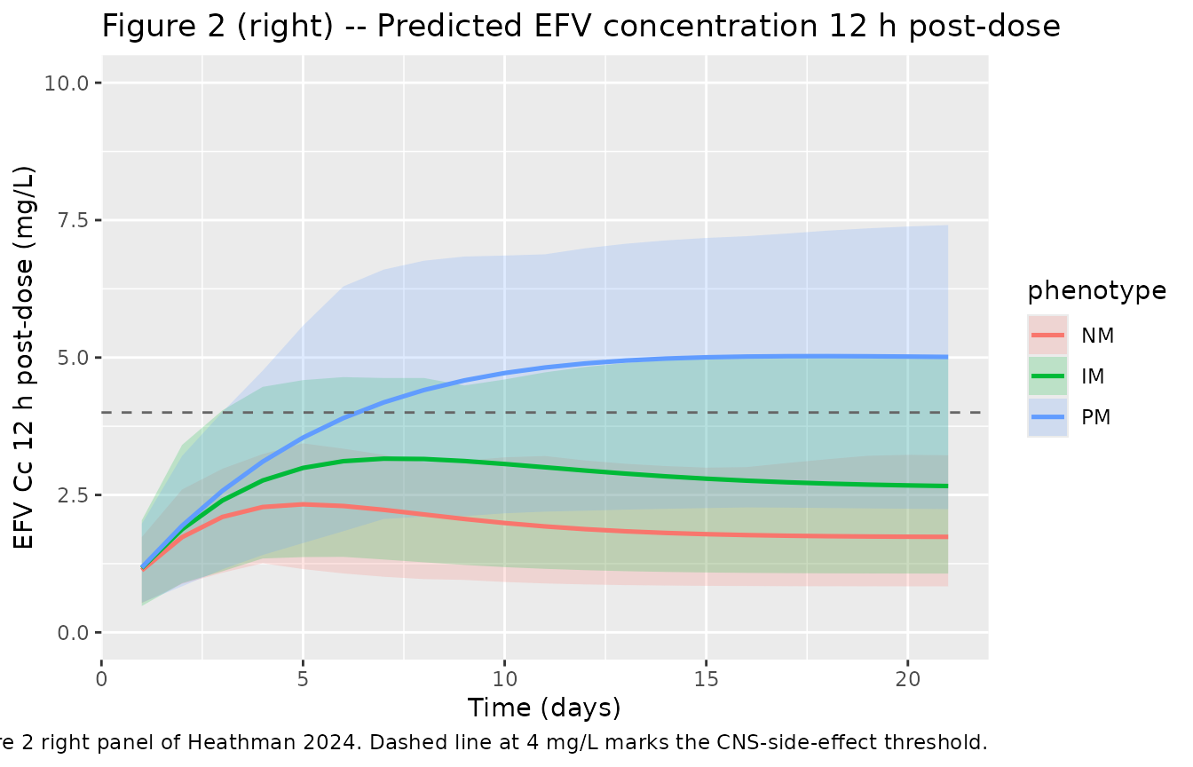
The replicated trajectory recovers the paper’s qualitative findings: NM and IM peak around days 5-10 then decline as CYP2B6 autoinduction lowers EFV clearance to its induced steady state, while PM continues to accumulate through days 14-21 because the CYP2B6 Emax is reduced by 93.2% and there is essentially no autoinduction.
Figure 3 – Predicted Steady-State EFV Concentrations
Heathman 2024 Figure 3 shows the steady-state (final day) EFV concentration profile by phenotype across the 24 h dosing interval, and a box-plot of the 12-h-post-dose steady-state concentration by phenotype. We reproduce the left panel (the dosing-interval profile on day 21).
day21 <- sim_vpc |>
  dplyr::filter(time >= 24 * 20, time <= 24 * 21) |>
  dplyr::mutate(t_post = time - 24 * 20) |>
  dplyr::group_by(phenotype, t_post) |>
  dplyr::summarise(
    q05 = quantile(Cc, 0.05, na.rm = TRUE),
    q50 = quantile(Cc, 0.50, na.rm = TRUE),
    q95 = quantile(Cc, 0.95, na.rm = TRUE),
    .groups = "drop"
  )

ggplot(day21, aes(x = t_post, colour = phenotype, fill = phenotype)) +
  geom_ribbon(aes(ymin = q05, ymax = q95), alpha = 0.20, colour = NA) +
  geom_line(aes(y = q50), linewidth = 0.9) +
  labs(x = "Time post-dose on day 21 (h)",
       y = "EFV plasma concentration (mg/L)",
       title = "Figure 3 (left) -- Day-21 EFV dosing-interval profile by phenotype",
       caption = "Replicates Figure 3 left panel of Heathman 2024.")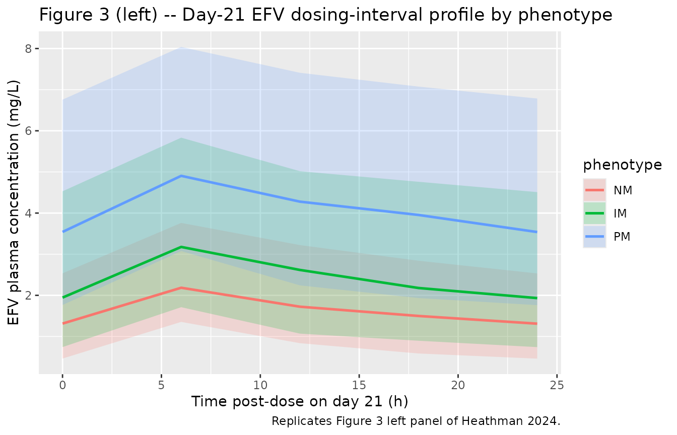
ss_t12 <- sim_vpc |>
  dplyr::filter(time == 24 * 21 - 12)

ggplot(ss_t12, aes(x = phenotype, y = Cc, fill = phenotype)) +
  geom_boxplot(alpha = 0.5, outlier.size = 0.7) +
  geom_hline(yintercept = 4, linetype = "dashed", colour = "grey40") +
  geom_hline(yintercept = 1, linetype = "dotted", colour = "grey40") +
  labs(x = "CYP2B6 phenotype",
       y = "EFV Cc 12 h post-dose on day 21 (mg/L)",
       title = "Figure 3 (right) -- Steady-state EFV at 12 h post-dose by phenotype",
       caption = paste0("Replicates Figure 3 right panel of Heathman 2024. ",
                        "Dashed line: 4 mg/L CNS-side-effect threshold; ",
                        "dotted line: 1 mg/L minimum effective concentration."))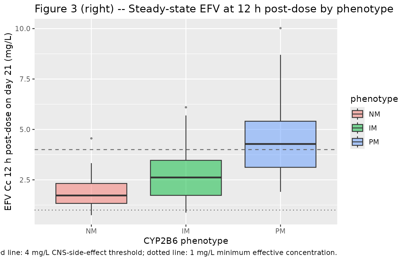
Quick sanity check of the paper’s headline claim (“steady-state concentrations 12 hours post-dose exceed 4 mg/L in 58% of PM subjects”):
ss_t12 |>
  dplyr::group_by(phenotype) |>
  dplyr::summarise(
    n              = dplyr::n(),
    median_mg_L    = round(median(Cc, na.rm = TRUE), 2),
    pct_above_4    = round(100 * mean(Cc > 4, na.rm = TRUE), 1),
    pct_below_1    = round(100 * mean(Cc < 1, na.rm = TRUE), 1),
    .groups = "drop"
  ) |>
knitr::kable(caption = "Day-21 12 h-post-dose EFV exposure by CYP2B6 phenotype (simulated cohort).")| phenotype | n | median_mg_L | pct_above_4 | pct_below_1 |
|---|---|---|---|---|
| NM | 60 | 1.72 | 1.7 | 10.0 |
| IM | 60 | 2.62 | 11.7 | 3.3 |
| PM | 60 | 4.28 | 55.0 | 0.0 |
PKNCA validation
Heathman 2024 does not publish a structured NCA table; the validation here covers the steady-state interval (day 21) Cmax / Tmax / AUC / half-life by phenotype using PKNCA. We use only the EFV Cc output (the parent analyte) because that is what the paper’s clinical-exposure narrative is built on.
sim_nca <- sim_vpc |>
  dplyr::filter(time >= 24 * 20, time <= 24 * 21) |>
  dplyr::mutate(time_post = time - 24 * 20) |>
  dplyr::filter(!is.na(Cc)) |>
  dplyr::select(id, phenotype, time_post, Cc)

# Guarantee a time = 0 row (start of the day-21 interval) per (id, phenotype).
sim_nca <- dplyr::bind_rows(
  sim_nca,
  sim_nca |> dplyr::distinct(id, phenotype) |>
    dplyr::mutate(time_post = 0, Cc = NA_real_)
) |>
  dplyr::distinct(id, phenotype, time_post, .keep_all = TRUE) |>
  dplyr::arrange(id, time_post)

# Use the first measured Cc as the steady-state pre-dose concentration so AUC
# starts at the actual concentration rather than a forced zero.
sim_nca <- sim_nca |>
  dplyr::group_by(id, phenotype) |>
  dplyr::mutate(Cc = ifelse(is.na(Cc) & time_post == 0, Cc[!is.na(Cc)][1], Cc)) |>
  dplyr::ungroup()

conc_obj <- PKNCA::PKNCAconc(sim_nca, Cc ~ time_post | phenotype + id)

dose_df <- data.frame(
  id        = sort(unique(sim_nca$id)),
  time_post = 0,
  amt       = 600,
  phenotype = sim_nca |>
    dplyr::distinct(id, phenotype) |>
    dplyr::arrange(id) |>
    dplyr::pull(phenotype)
)
dose_obj <- PKNCA::PKNCAdose(dose_df, amt ~ time_post | phenotype + id)

intervals <- data.frame(
  start       = 0,
  end         = 24,
  cmax        = TRUE,
  tmax        = TRUE,
  auclast     = TRUE,
  half.life   = TRUE
)

nca_data <- PKNCA::PKNCAdata(conc_obj, dose_obj, intervals = intervals)
nca_res  <- PKNCA::pk.nca(nca_data)

nca_summary <- as.data.frame(nca_res$result) |>
  dplyr::filter(PPTESTCD %in% c("cmax", "tmax", "auclast", "half.life")) |>
  dplyr::group_by(phenotype, PPTESTCD) |>
  dplyr::summarise(median = median(PPORRES, na.rm = TRUE),
                   q05    = quantile(PPORRES, 0.05, na.rm = TRUE),
                   q95    = quantile(PPORRES, 0.95, na.rm = TRUE),
                   .groups = "drop") |>
  dplyr::mutate(across(c(median, q05, q95), \(x) round(x, 3))) |>
  tidyr::pivot_wider(names_from = PPTESTCD, values_from = c(median, q05, q95))

knitr::kable(
  nca_summary,
  caption = paste0("Day-21 PKNCA summary for EFV plasma concentrations by ",
                   "CYP2B6 phenotype (median and 5th-95th percentile across ",
                   "the simulated cohort). Cmax in mg/L; AUC0-24 in ",
                   "mg-h/L; half-life in h.")
)| phenotype | median_auclast | median_cmax | median_half.life | median_tmax | q05_auclast | q05_cmax | q05_half.life | q05_tmax | q95_auclast | q95_cmax | q95_half.life | q95_tmax |
|---|---|---|---|---|---|---|---|---|---|---|---|---|
| NM | 39.724 | 2.185 | 30.840 | 6 | 20.300 | 1.354 | 12.702 | 6 | 74.181 | 3.761 | 68.843 | 6 |
| IM | 60.481 | 3.177 | 35.591 | 6 | 26.497 | 1.712 | 18.464 | 6 | 118.044 | 5.833 | 89.258 | 6 |
| PM | 101.310 | 4.905 | 56.569 | 6 | 55.445 | 3.077 | 25.884 | 6 | 174.311 | 8.039 | 146.727 | 6 |
The Heathman 2024 poster does not report a published NCA table to compare against, so the table above stands on its own as a sanity check of the day-21 exposure metrics by phenotype.
Assumptions and deviations
- The Heathman 2024 poster does not publish baseline demographics
(age, weight, sex, race, ethnicity). The
populationmetadata records these as “not reported in the conference poster” and the validation cohort uses three equal-sized arms (NM / IM / PM) with no other covariate stratification. - Heathman 2024 reports
EC50-2B6 = 32000 nMandEC50-2A6 = 12500 nM. The model stores both EC50 values inmg/L(=ug/mL) so they share units with the EFV plasma concentration. The conversion uses the EFV molecular weight 315.68 g/mol (C14H9ClF3NO2), givingEC50-2B6 = 10.10 mg/LandEC50-2A6 = 3.95 mg/L. The conversion is documented inline inini(). - Heathman 2024 reports “% reduction” for the CYP2B6 phenotype effects
on CL-EFV,2B6 and EMAX-2B6 (IM 9.72% / 53.5%; PM 9.06% / 93.2%). The
model encodes these as multiplicative log-scale shifts via the canonical
e_<cov>_<param>covariate-effect parameters, with NM as the reference category (both CYP2B6_IM and CYP2B6_SM equal to 0). Heathman’s “PM” maps to the canonicalCYP2B6_SM(slow / poor metabolizer); see the in-filecovariateDatanotes and the precedent inRobarge_2017_efavirenzandBienczak_2016_nevirapine. - The CIs on
CL-EFV,2B6IM and PM reductions cross zero (the IM CI is -2.85 to 20.8 and the PM CI is -12.7 to 26.6 per Table 1). The point estimates are retained as reported. The EMAX-2B6 reductions are clearly significant for both IM (CI 37.1-65.6) and PM (CI 87.6-96.3). - Heathman 2024 fixes the central volume of both metabolites (Vc-8OH
and Vc-7OH) equal to Vc-EFV because of identifiability. The model
encodes this as
vc_8oh <- vc; vc_7oh <- vcinmodel(). No separate ini parameter is created for the metabolite central volumes. - The parent-to-metabolite formation flux is treated as direct mass
transfer in the apparent-volume parameterisation:
d/dt(central_8oh) = cl_2b6 * enzyme_2b6 / vc * central - .... The EFV molecular weight (315.68 g/mol) is similar to the metabolite MWs (8-OH and 7-OH each add 16 g/mol, so MW ratio ~ 1.05); the small ratio is absorbed into the apparent clearance terms per standard popPK metabolite-modelling convention. - The poster does not report IIV correlations between any pair of PK
or autoinduction parameters; all IIVs in this model are diagonal. The
15.1% CV FIXED entries appear on UGT- and several minor metabolite arms;
they are encoded with
fixed()wrappers so a downstream user does not refit them. - This vignette uses 60 subjects per phenotype arm (180 total) to keep the render time comfortably below 5 minutes; the paper’s actual cohort was 135 (allocation across NM/IM/PM not specified in the poster).
New canonical names registered with this extraction
This extraction adds the following canonical entries to the
convention registry (inst/references/compartment-names.md
and inst/references/parameter-names.md). They are reviewed
alongside the model file and vignette in the same PR; the underlying
mechanism – parallel isoenzyme autoinduction, CYP-isoenzyme-partitioned
clearance – generalises to future autoinduction popPK papers
(rifampicin-induced CYP3A4, ritonavir CYP3A4 inhibition, isoniazid NAT2
induction).
| Register file | New canonical entry | Type | Role |
|---|---|---|---|
compartment-names.md |
enzyme_2b6 |
compartment | Parallel CYP2B6 enzyme pool (extends the single-enzyme
Wicha 2018 form) |
compartment-names.md |
enzyme_2a6 |
compartment | Parallel CYP2A6 enzyme pool |
compartment-names.md |
8oh |
metabolite-suffix | 8-hydroxy-efavirenz metabolite (parallel to the existing
3oh agomelatine precedent) |
compartment-names.md |
7oh |
metabolite-suffix | 7-hydroxy-efavirenz metabolite |
parameter-names.md |
lcl_2b6 / cl_2b6
|
log-pk / bare-pk | CYP2B6-mediated metabolic clearance arm (multiplied by
enzyme_2b6(t)) |
parameter-names.md |
lcl_2a6 / cl_2a6
|
log-pk / bare-pk | CYP2A6-mediated metabolic clearance arm |
parameter-names.md |
lcl_ugt / cl_ugt
|
log-pk / bare-pk | UGT-mediated metabolic clearance arm (not autoinduced in the founding example) |
parameter-names.md |
ld1 / d1
|
log-pk / bare-pk | Zero-order absorption duration; codifies the precedent already used
in Aouri_2017_rilpivirine.R and
Goggin_2004_emfilermin.R
|
After registration,
checkModelConventions("Heathman_2024_efavirenz") reports no
errors or warnings.